Using PEAK to measure
The default measurement software on the Bloch A endstation is SES, but adventurous users may wish to start using prototype implementations of acquisitions using the new ScientaOmicron ‘PEAK’ software.
The information below is valid as of December 2025
Advantages of PEAK:
A fully-featured python API enables advanced measurement modes, including fast spatial mapping and sequences of arbitrary complexity (including integration of undulator and temperature control).
‘DFS’ mode allows 3D adjustment of the analyzer focal position entirely in software, meaning you do not have to move the sample in order to optimize focus. Great for samples with very small domains.
Disadvantages of PEAK:
With the exception of spatial mapping modes: less straightfoward, stable and user-friendly than SES
Native user interface much is much more cumbersome than SES for live sample alignment
Advanced measurement modes currently require being comfortable with basic python scripting
New file saving format (NeXuS-style HDF5) may require updated file loaders for your analysis software
Getting PEAK ready to measure
Close SES completely - it is not possible for PEAK and SES to simultaneously connect to the analyzer or camera
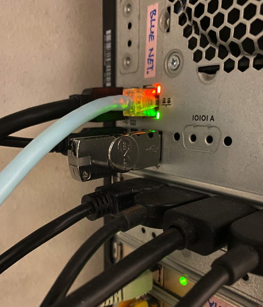
The Wibu CodeMeter USB dongle must be installed in the measurement computer. It is usually left in permanently
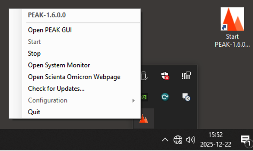
If the PEAK service has not already started, launch it from the desktop icon (“Start PEAK 1.6.0.0 Application”)
A PEAK icon is now present in the system tray (next to the clock in the bottom right corner). Right click on it and choose “Open PEAK GUI”
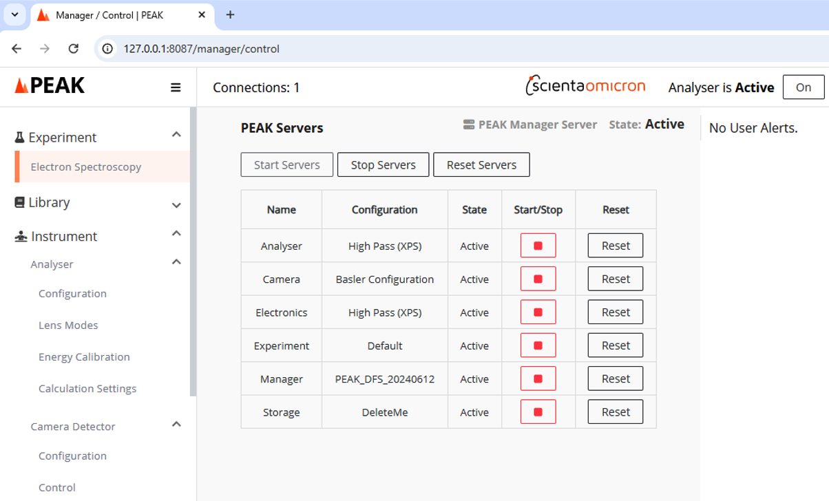
The PEAK GUI appears in a new browser tab. The default configuration “PEAK_DFS_20240612” should be listed on this “PEAK Servers” page
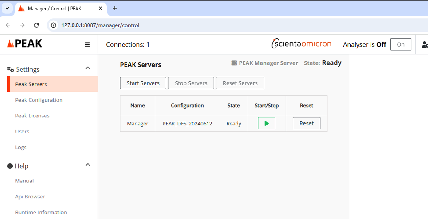
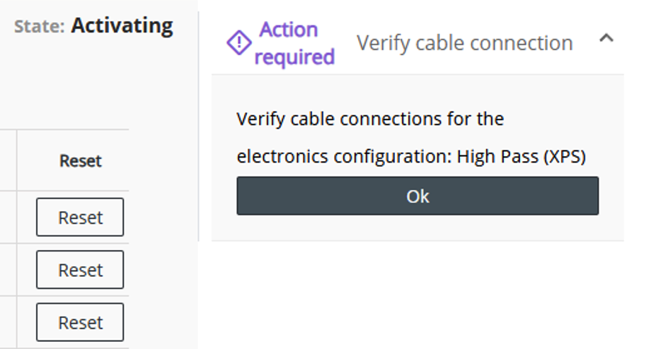
Click on “Start Servers” (This is the point at which SES must be disconnected, and SES cannot be reconnected until you have pressed “Stop Servers”). You will be prompted to confirm cable connections for High Pass (XPS), choose OK.
Press all green play buttons on the Electronics, Camera and Analyser servers until all servers are in the state “Active”
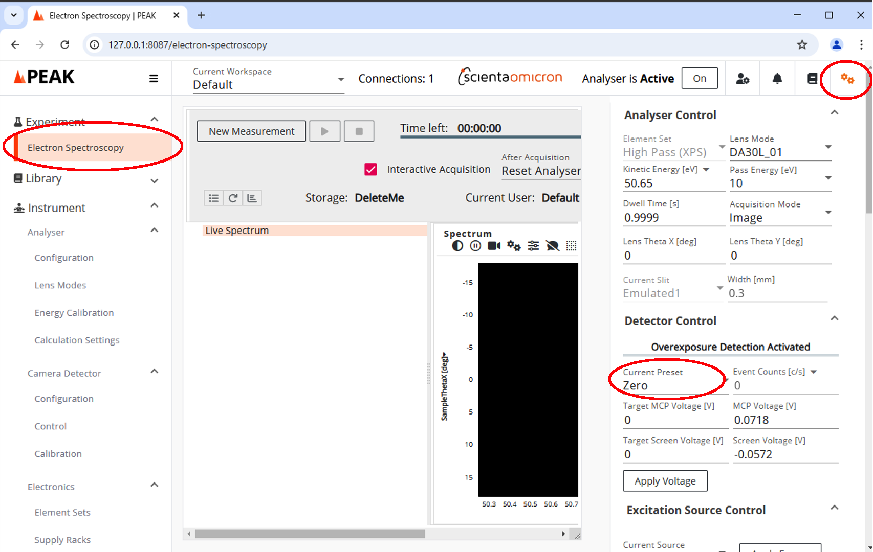
On the left hand pane, choose “Electron Spectroscopy” under “Experiment”
In the extreme upper right corner, click on the gear icons. You are now in ‘live view’ mode and can choose appropriate analyzer settings then run up the MCP (change “Current Preset” to “Calibrated”).
Switching back to SES
Go back to the Settings>Peak Servers tab on the left-hand panel of the PEAK GUI. Press the ‘stop servers’ button and ensure all servers have shut down. Nothing else is required - you can now re-launch and use SES.
Performing a measurement with the blochPEAK library
Documentation for the blochPeak library can be found here: ((coming soon!))
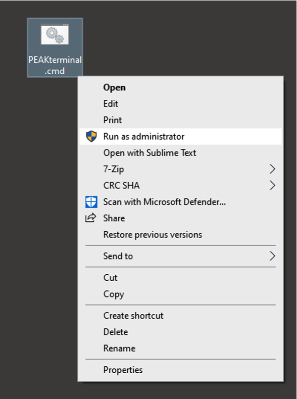
There is a batch file on the desktop (“PEAKterminal.cmd”). You must right-click and launch this as administrator, and as of writing the default bloch-user account does not have adminstrator priviledges. Until this is resolved, a bloch staff member must help you to launch this. If you don’t launch as admin, things will appear to work at first but will fail when you try to perform an acquisition (‘brotli: decoder failed’ error).
This will open a new terminal window in which the PEAK python environment is correctly configured. Within this terminal window, navigate to wherever you want the data to end up - for example, this might be your experiment folder on the network drive:
t:
cd 20250666/2025121212/raw
Copy a new blank PEAK notebook into the same folder. This is found at T:/bloch/BlankPEAKNotebook.ipynb
Within the terminal window, launch a jupyter notebook server (jupyter notebook) and open that notebook. You can perform all acquisitions from within this notebook.
Here is an example of setting up and performing a swept E-k 2D measurement:
import blochpeak as bp
config = bp.swept.configureAnalyzer(energyRange=[131.6,136.3],stepSize_meV=100,passEnergy=20)
scan = bp.swept.go(config)
bp.disconnect(config)
While a more complicated sequence of taking two different measurement at each point in a photon energy scan might look like this:
import blochpeak as bp
swept_config = bp.swept.configureAnalyzer(energyRange=[131.6,136.3],stepSize_meV=100,passEnergy=20)
da30_config = bp.deflectormap.configureAnalyzer_fixed(centerEnergy=135.6,deflectorRange=[-15,15],deflectorStep_deg=1,passEnergy=20,dwell_s=0.5)

for hv in np.arange(start=30,stop=50,step=5):
  bp.set_hv(hv)
  bp.swept.go(swept_config,numSweeps=1)
  bp.deflectormap.go(da30_config,numSweeps=1)

bp.disconnect(swept_config)
bp.disconnect(da30_config)
Spatial module
Two spatial-map modes are available: fast ‘flyscans’ and more precise ‘step scans’. Both acquire in fixed mode only.
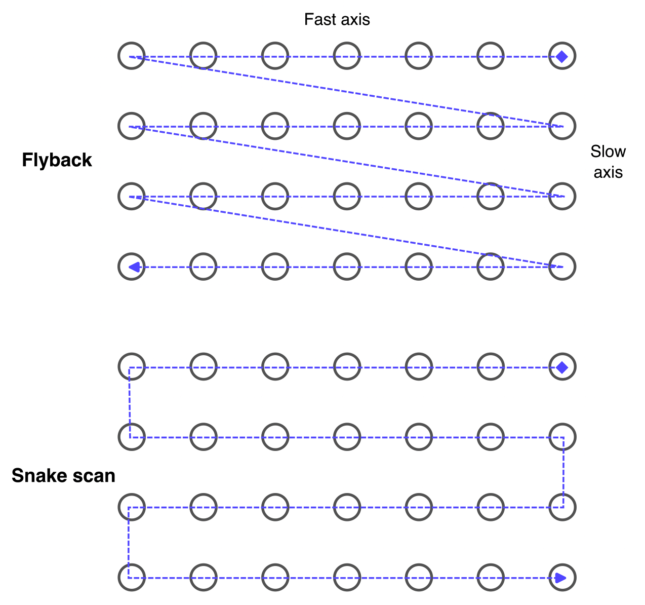
Step scans move from point-to-point on a regularly spaced grid of points. Acquisition occurs at each data point, never when moving between data points. This scan style is appropriate when long (>1s) integration times are needed per point, and/or when the accuracy of the spatial information is very important. We can define a fast-scan axis and a slow-scan axis according to the image below:
In cases with looser requirements (e.g. large-area scans to coarsely map out the sample), the ‘dead time’ associated with point-by-point motion becomes problematic. Flyscans address this. During each fast-axis scanline we begin a continuous linear motion and while it is moving, continuously stream measurement spectra into memory. Each spectrum is tagged with the manipulator coordinates at the time of acquisition. To link scanlines we can choose to either perform a traditional ‘jumpback’ raster scan, or a slightly more efficient ‘snake-scan’.
The minimum integration time is set by the camera frame rate (17 FPS / 59ms), while the maximum practical frame rate for fast flyscans is approximately 500ms. The spatial resolution depends on this sampling rate and on the manipulator velocity: fast acquisition and slow scan velocity gives the highest spatial resolution. There is a calculator function in the blochPEAK package to help you decide on the settings to use.
At the conclusion of either type of scan we will have a 1D array containing a few-thousand individual spectra and their (x,y) coordinates. For flyscans these will not directly to a regularly spaced grid, but we need them to be in order to visualize the map. A dedicated function interpolateToGrid() handles this re-mapping internally when you either call spatialmap.load() to load the saved file into memory as a pesto spectrum, or you trasnform and re-export the saved file with spatialmap.exportInterpolated()
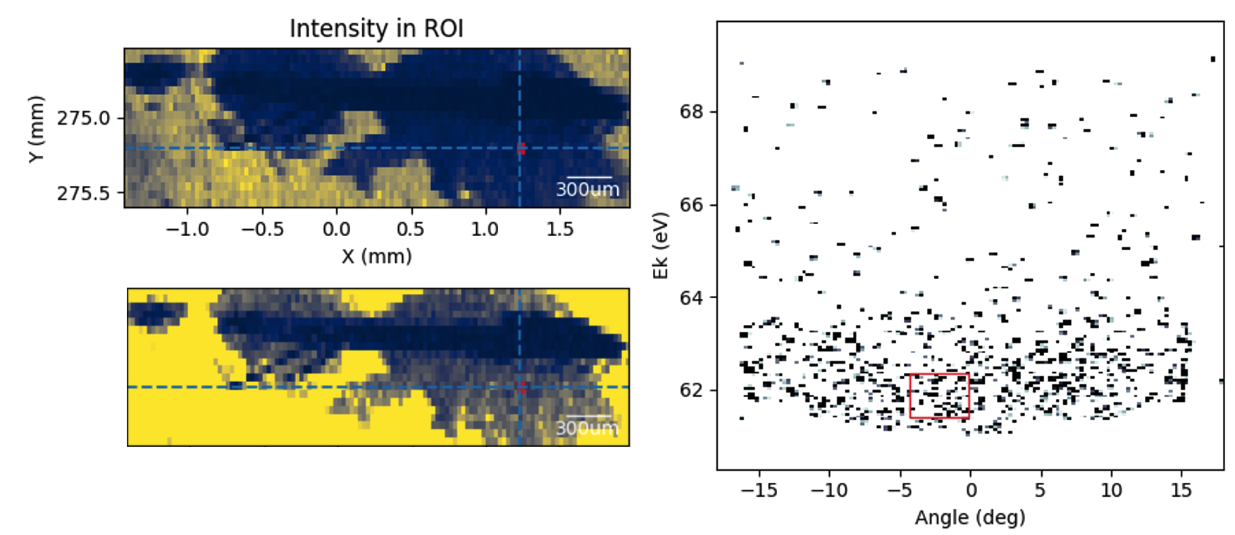
Below is an example flyscan measurement that obtains an overview of the entire sample with 30μm resolution. Once we have located a region of interest, we can zoom in and perform a more precise and lower noise stepscan to find optimal measurement positions.
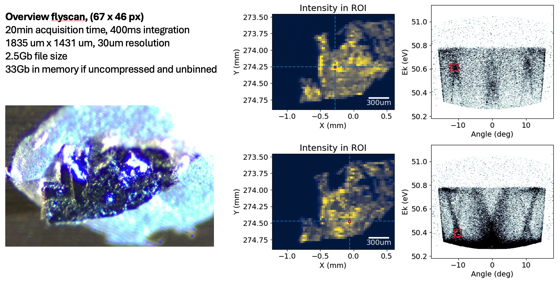
Flyscan maps can be extremely effective at picking out structure in extremely noisy spectra that would otherwise go completely unnoticed when moving around the sample manually. Individual frames here look little different to noise, but the final spatial map clearly resolves the Cu sample plate, the Ag epoxy and the needle-like sample. In this case the cleave was bad and there were no bands to find, but a map like this gives confidence that the beam is really positioned on the sample and the sample is just bad, rather than wondering if you have simply not found the sample yet.
Notes/considerations:
at the end of every scan-line, measurement data is saved to disk. This avoids overflowing memory, and means that if the scan is terminated early then all acquired data up until the end of the last completed scan-line will be safe.
Writing to disk takes a small amount of time, which can start to matter for fly-scans with dense sampling per scanline. In snake-scans the scan pauses at the end of each scan-line to complete this file write. In traditional jump-back scans, the writing occurs while the manipulator is doing the jump-back. This can reduce the speed advantage of snake-scans
traditional jump-back scans also have the advantage of backlash compensation, ensuring scan-lines are aligned.
flyscans are only continous and efficient along the fast-axis scanlines. The slow-axis motion is still stepped
all spatial maps are obtained at the full detector resolution, and saved in a compressed format. As the data is de-compressed when loaded into memory for viewing, it can easily consume more memory than is available. Binning can and usually should be applied at the point of loading or re-exporting the data
Known issues
The countrate is not equivalent between SES and PEAK. It is safest to check the countrate first in SES before switching to PEAK.
PEAK has built-in overexposure protection that will shut down the detector if the maximum countrate is grossly exceeded. Recovery from an overexposure event often requires restarting the analyzer server in PEAK
When using a DFS configuration in PEAK there will be an error message about detector retardation that is not present in non-DFS configurations. The cause and implications of this have not yet been determined
We have not yet performed full energy calibration checks, so there may be small discrepancies between measurements performed in SES and PEAK. Similarly, we have not yet investigated the performance of the straight-slit correction.
If an aquisition does not terminate normally, the analyzer might get stuck in the wrong state in PEAK (e.g. Measuring instead of Active). Go into the Settings>Peak Servers page in the PEAK UI and reset the Analyser server if this happens.