Using Prodigy to measure

By default, all data will be contained within a single *.sle file, which can only be accessed by Prodigy. We typically then manually export completed measurements to .xy files, named after the scan ID number. Auto-exporting to xy is enabled by default, but as the file name convention is based purely on the time of the measurement, this is not especially helpful.

Device controls panel

This is where you connect to and control analyzer hardware. When first aligning, you will be working in the PhoibosCCD panel and watching the live camera feed - this is the equivalent of Voltage Calibration mode in SES.

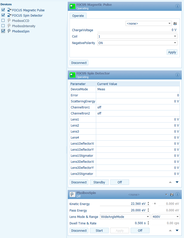
For regular ARPES, you will connect exclusively to the device PhoibosCCD. When working with the spin detector, you will disconnect from PhoibosCCD and instead connect to PhoibosSpin, FOCUS Magnetic Pulse and FOCUS Spin Detector. Connecting and disconnecting is accomplished via the checkboxs in the device list on the left.

Device	What is it?	When is it used?
FOCUS Magnetic Pulse	Control unit for target magnetization in spin detector	Spin ARPES
FOCUS Spin Detector	Control unit for spin detector	Spin ARPES
PhoibosCCD	MCP/CCD camera	Normal ARPES
PhoibosIntensity	Total intensity (pre-scattering) channeltron in spin detector	Never
PhoibosSpin	Scattered intensity channeltron in the spin detector	Spin ARPES

Experiment editor panel

This is where you can configure, acquire and save measurements. In a loose sense it is similar to the SES ‘sequence editor’.

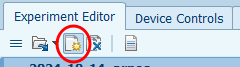
Begin by creating a new experiment file (*.sle):

New experiments (*.sle files) are placed by default in offline1/staff/bloch/spin_station/, and by default are named after the current date. On the local computer, this is mapped to Q:/spin_station. When creating the file, choose the bottom option, ‘Experiment from Scratch’.

In the new, empty experiment file add a new measurement by pressing the bottom-most plus icon:

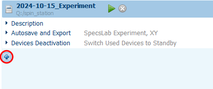
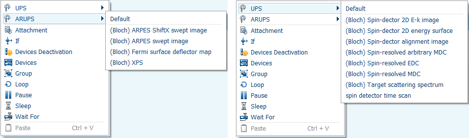
and then choosing a measurement template. Templates exist for all common measurement types, and we highly recommend that you construct your measurements from these starting points rather than from scratch. Spin templates are under ‘UPS’ while regular ARPES templates are under ‘ARUPS’. All the official beamline templates are prefixed with ‘(Bloch)’, but you are free to create your own as well.

Configuring measurements:

Note

It is not possible to view all configuration parameters for a measurement at the same time - you will need to click on the blue top-level bars (anything with a checkbox on the left hand side) to make it expand and expose its parameters.

Top level:

PhoibosCCD (regular ARPES): Here you can define a ShiftX/ShiftY deflector offset, and the number of energy and angle channels. Full detector resolution is 1392x1040, but to keep file sizes manageable it is more typical to use something like 200x200 (fixed mode deflector maps) or 300x600 (swept 2D cuts)

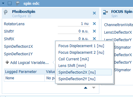
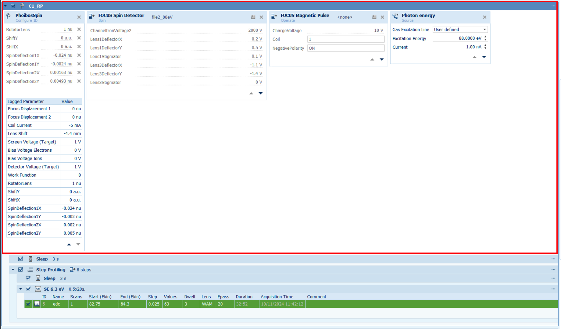
PhoibosSpin (spin ARPES): Here you specify the spin rotator setting (+/- 1) and the ShiftX/ShiftY deflector offset. We also strongly recommend including the lens voltages SD1X,SD1Y,SD2X and SD2Y. Those values are always initialized to whatever is currently set in the PhoibosSpin device panel, but you can manually choose different values.

FOCUS Spin Detector: Here you specify the L1 and L3 lens voltages. The preferred way of doing this is to load a previously saved configuration file, by clicking on the disk icon

FOCUS Magnetic Pulse: Define the initial magnetization direction of the target. by choosing a coil (1 or 2) and a polarity.

Photon energy: An excitation source is required to be present for each measurement, but the values are only used for metadata.

Spectrum definition (lowest level):

Here you define the actual scans. Multiple scans can be defined within a spectrum group, but they will all use the same device and analyzer configurations (ShiftX, rotator, scan mode…). If you want to change any of these, you need to make an entirely new measurement entry in the experiment editor.

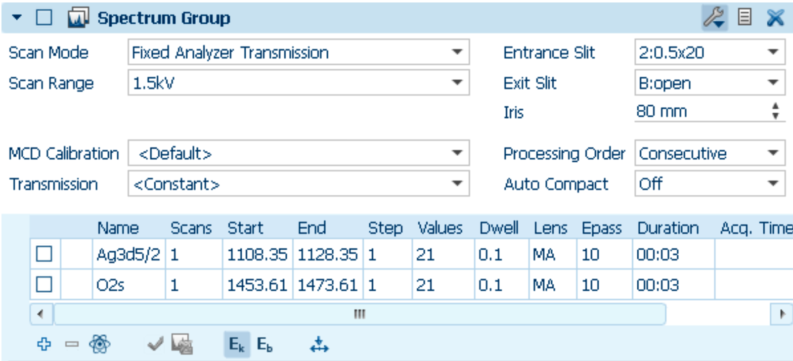
Scan Mode: Use ‘Fixed Analyzer Transmission’ for measurements that sweep the energy axis. Use ‘Snapshot’ for snapshot modes (e.g. efficient Fermi surface maps). Use ‘Fixed energy’ for Spin MDCs.

Scan Range: The maximum range of the Phoibos high voltage supply. Strictly speaking this should be the lowest range you can get away with, to get the best resolution out of the digital-to-analog converters. In practice, the default is almost always fine.

MCD Calibration: How position on the CCD image is mapped to kinetic energy. These files are stored in C:\ProgramData\SPECS\SpecsLab Prodigy\Database\DatasetCalib1D. Leave this as the default value.

Transmission: Adjustments to intensity vs energy for the scan. Leave this as the default (‘<Constant>’)

Entrance Slit / Exit Slit / Iris: Unimportant (purely for metadata)

Processing Order: Leave as the default (‘Consecutive’)

Auto Compact: Should be ‘Off’

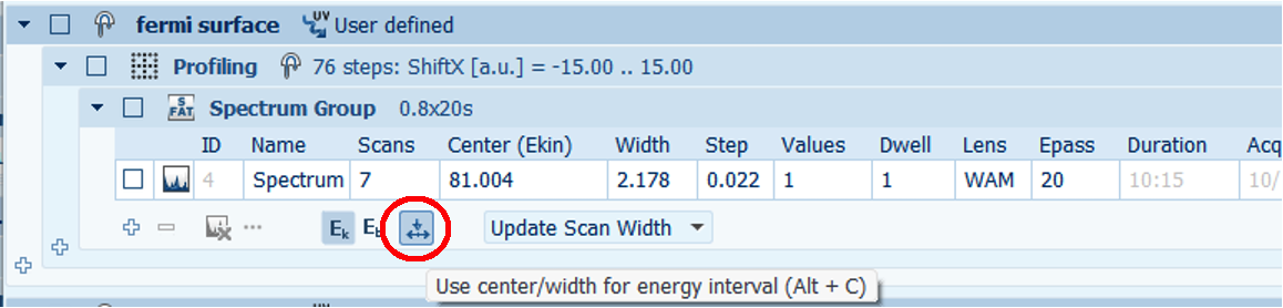
Good to know: When defining the energy range there is a button that toggles the UI between specifying start/end values (useful for swept modes) and center energy (useful for fixed modes)

Acquiring and saving measurements:

All measurements happen by defining them in the Experiment Editor, then enabling them (i.e. ticking the checkbox in the measurement definition), then pushing the green ‘play’ button at the top of the Experiment Editor window.

Once a measurement has been completed, it is automatically stored in the main .sle experiment file. To get your data out, right click on a completed measurement in the Experiment Editor window and export it as a .xy file.

Visualization panels

This discussion relates to data visualization within Prodigy. Once a measurement is finished it is also possible to export the data and visualize it in a Jupyter notebook.

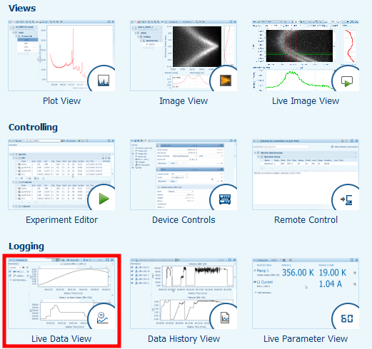
There are four different visualization panels you are likely to use in the course of a normal experiment:

Plot View is good for 1D data (XPS, spin EDC/MDCs)

Image View is for 2D and 3D datasets

Live Image View shows the live detector image, used when aligning the sample.

Live Data View Shows a time trace of countrate, used when optimizing lens voltages for the spin detector.

Viewing 3D deflector maps:

Viewing 1D and 2D datasets is hopefully self explanatory. Viewing 3D deflector maps is a bit more involved. From inside an Image View window:

1. Double click on the measurement you want to view. It should now have a tick next to it.

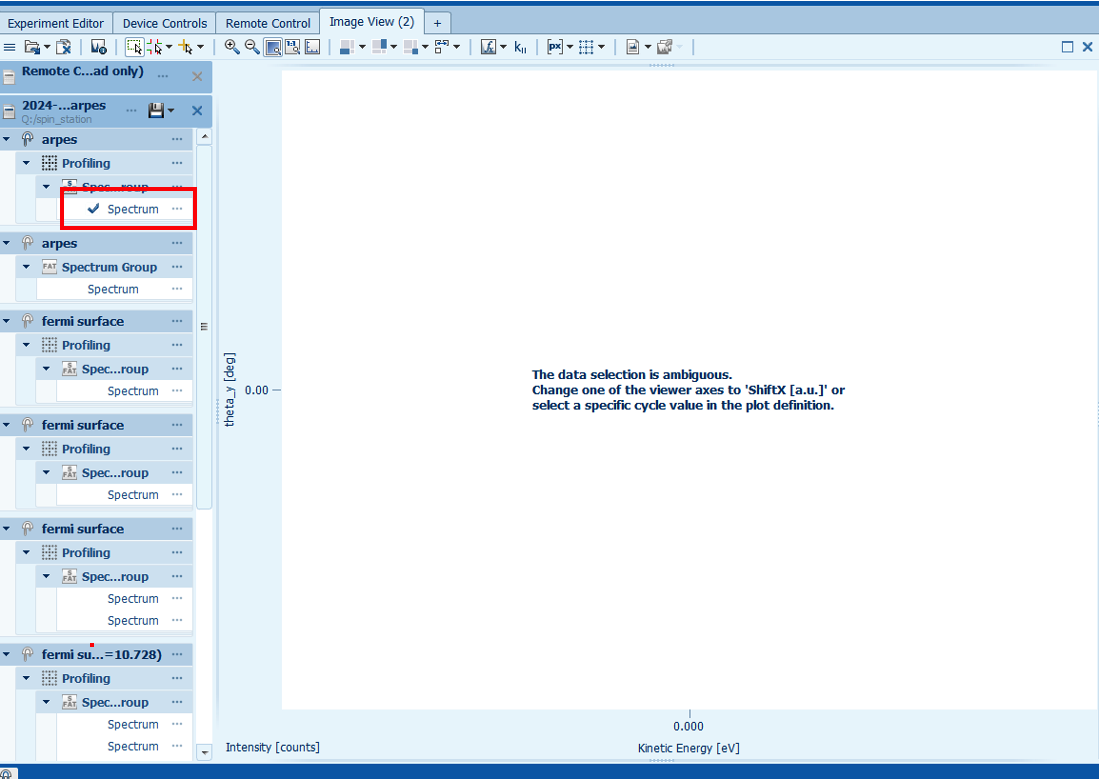
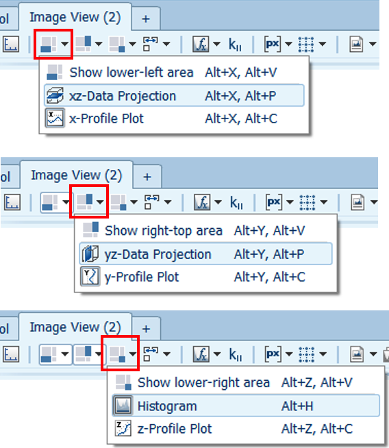
2. From the top bar, enable data projections on the lower and right sides, and the colormap histogram in the corner:

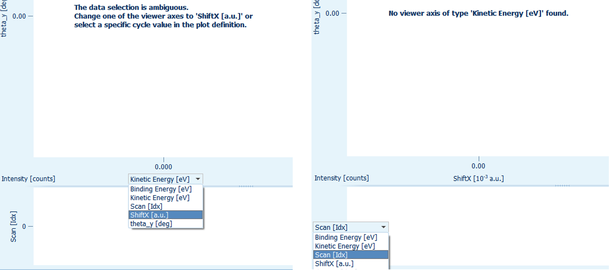
3. Changes the main plot x-axis to ‘ShiftX’, and the lower plot y-axis to ‘Kinetic Energy’:

4. Enable Range Cursor then click on one of the data cuts. Click and drag the center of a range cursor axis to change the value of the Energy/Angle/ShiftX cut being plotted. You can also expand the size of the range cursor to set the slice integration. If you don’t seem to be able to move the range cursor, this might be because the range is set to integrate the entire axis.

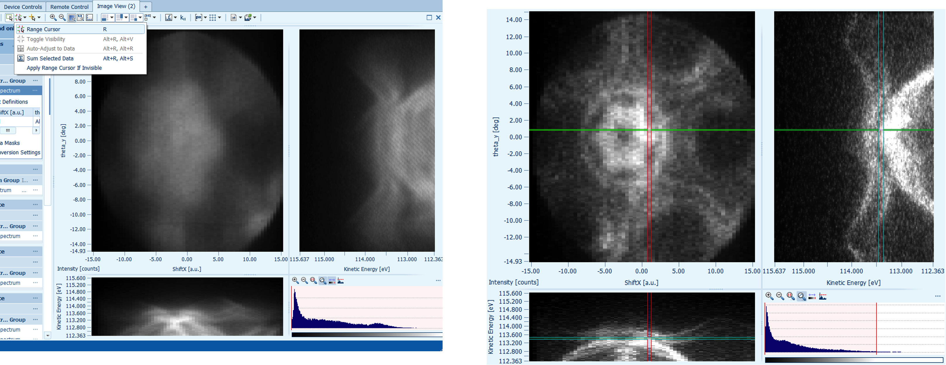
5. Adjust the colorscale using the Histogram in the lower right corner.

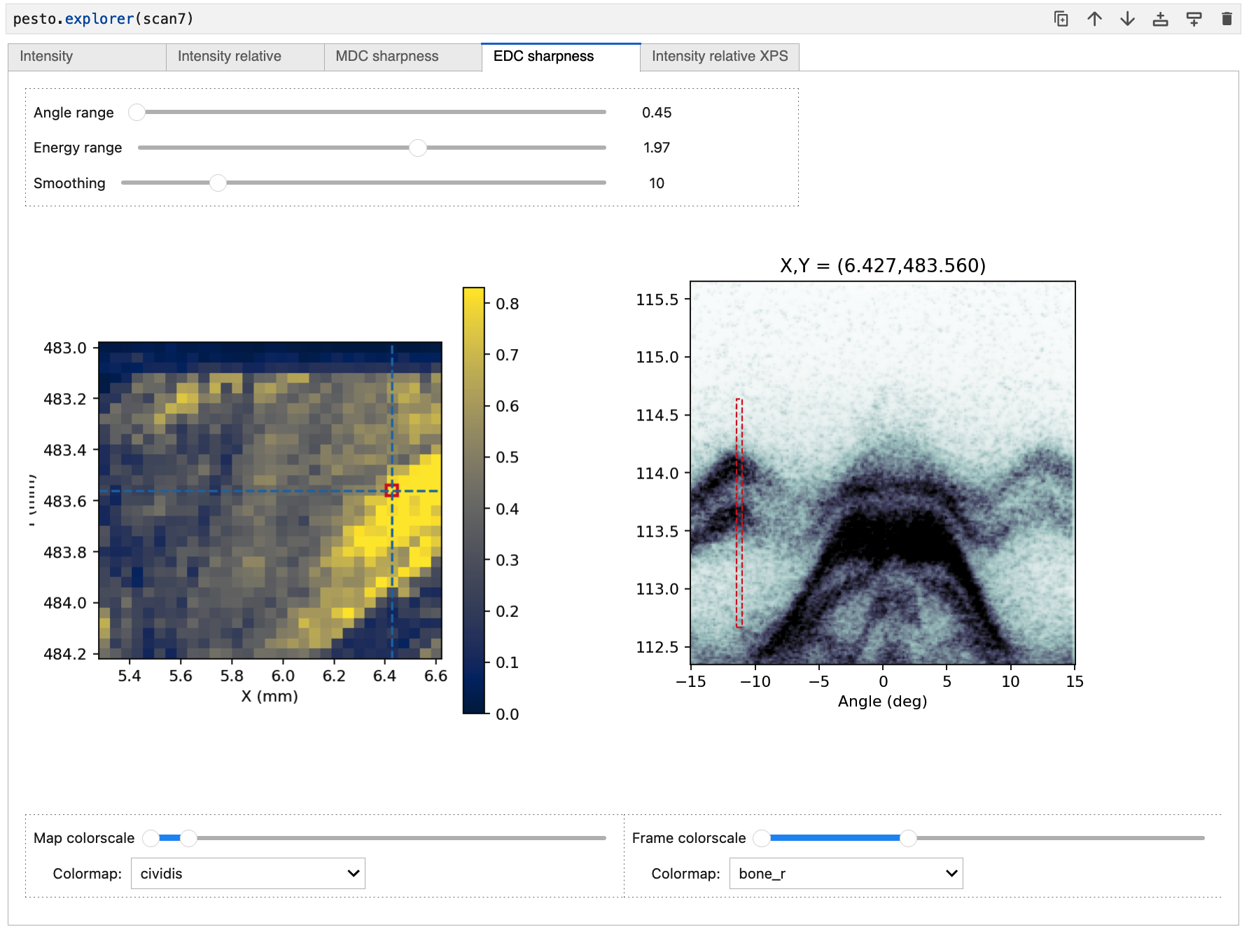
Spatial mapping

This is implemented by an external script, outside of the Experiment Editor.

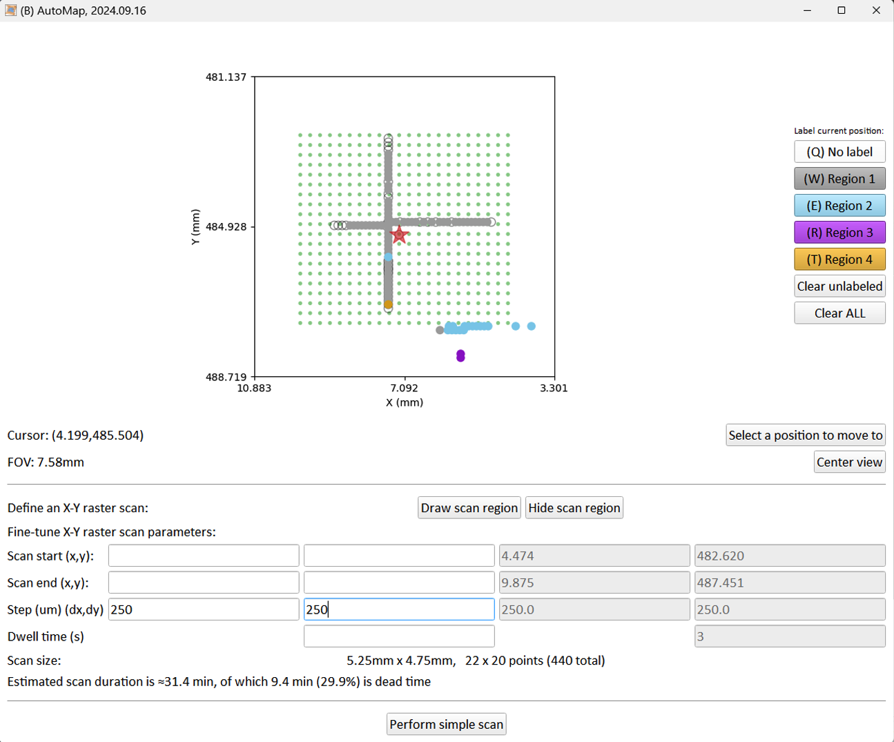
0. The easiest way to decide on the scan parameters and to monitor the scan progress is through the ‘AutoMap’ panel:

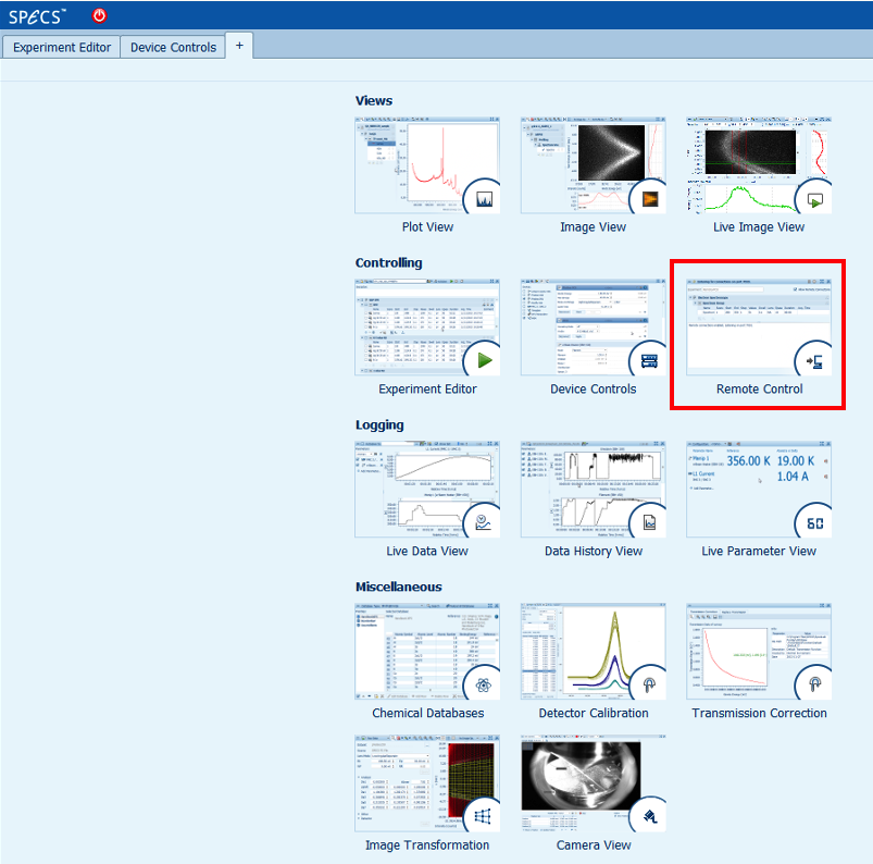
1. Open a new ‘Remote Control’ window in Prodigy:

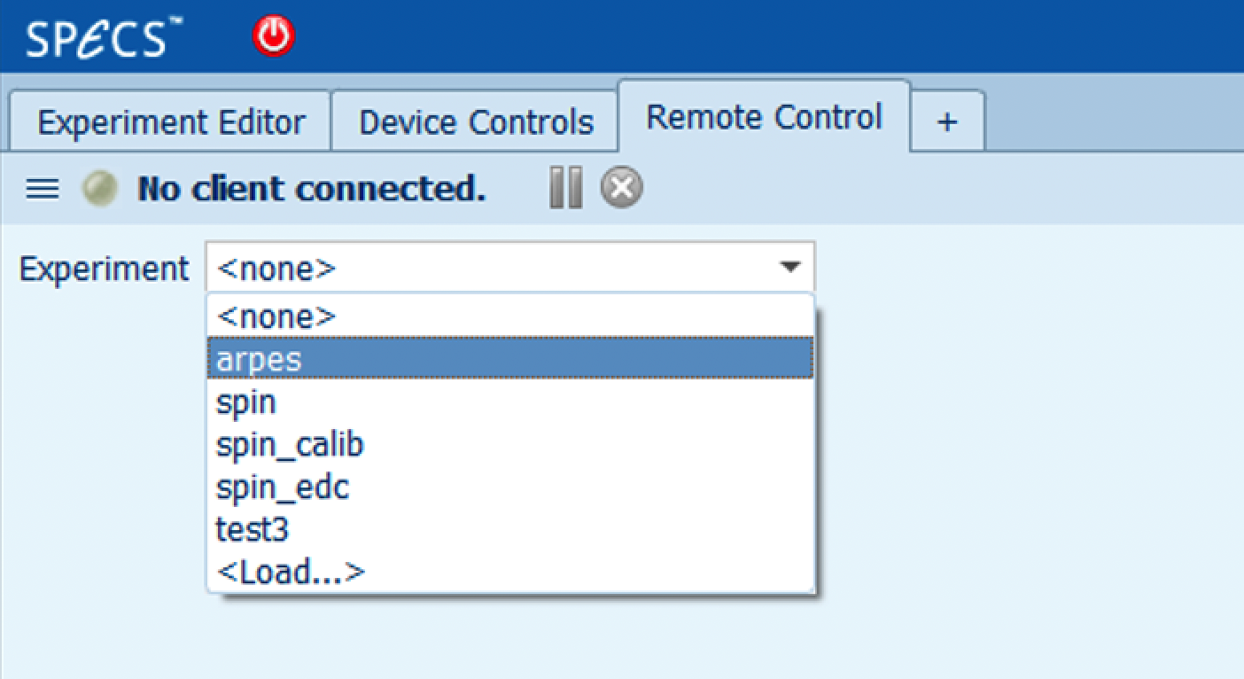
2. Load an ‘arpes’ experiment:

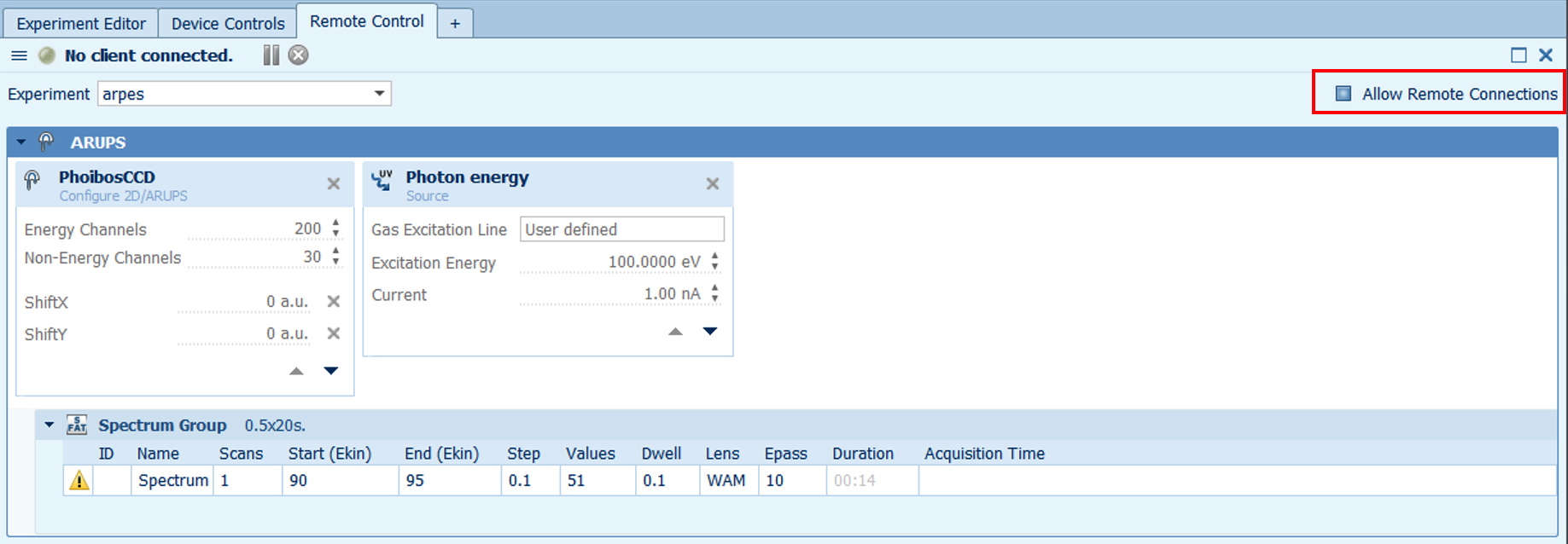
3. Check the ‘Allow Remote Connections’ box:

4. Launch the python script ‘spatial_map2.py’ by double clicking on it. This is located in C:\Users\bloch-user\Documents\Scripts\measurement. Fill in the X/Y start/stop/steps fields. Below that, configure the snapshot that will be acquired at each point.

Warning

The scan will crash if the frame size is too large compared to the dwell time. For example, a 300x300 frame size with 0.3s dwell will reliably crash. Suggested settings are 100x100 for fast scans (dwell 0.3s) and 300x300 for slower scans (>1.5s dwell).

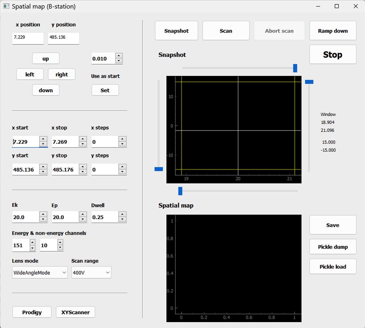
5. Check all required connections by pressing the ‘Prodigy’ and ‘XYScanner’ buttons on the bottom of the panel

6. Press the ‘Snapshot’ button on the top of the panel. This ramps up the detector voltages and acquires a single frame (you can see it in a Live Image View window in Prodigy). From this point onwards, the detector voltages remain ON.

7. Press the ‘Scan’ button to perform the XY-scan. The scan duration is currently about 15% larger than what the ‘AutoMap’ panel estimates.

8. When the scan finishes, the detector is still ramped up. Press the ‘Ramp down’ button.

9. The ‘Save’ button saves a simplified txt file containing integrated intensity. The ‘Pickle dump’ button saves the full dataset, in a format that can be loaded and viewed in a Jupyter notebook running pesto.

10. To return to normal operation using the Experiment Editor, uncheck the ‘Allow remote connection’ button in the ‘Remote Control’ window.

Optimizing spin detector lens voltages

Note

When optimizing the transmission, it is helpful to work with a high countrate - so choose a kinetic energy that results in a lot of electrons, and also consider temporarily opening up the beamline exit slits.

There are 10 lens voltages that typically need to be optimized before starting a spin experiment. This is important to do for successful spin measurements - the impact of these optimizations on the count rate can can easily be an order of magnitude, and optimal values can vary between different retarding ratios, rotator settings, and across the full ShiftX / ShiftY range.

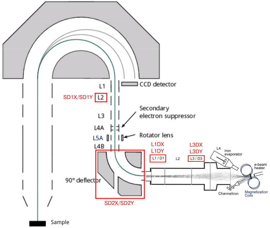
The lens voltages in question are listed below:

Name	Location	Power supply
SpinDeflection1X	Transfer lens, before spin rotator (L2)	Phoibos HSA
SpinDeflection1Y	Transfer lens, before spin rotator (L2)	Phoibos HSA
SpinDeflection2X	Transfer lens, inside the 90° bend	Phoibos HSA
SpinDeflection2Y	Transfer lens, inside the 90° bend	Phoibos HSA
Lens1DeflectorX	Spin detector	Spin controller
Lens1DeflectorY	Spin detector	Spin controller
Lens1Stigmator	Spin detector	Spin controller
Lens3DeflectorX	Spin detector	Spin controller
Lens3DeflectorY	Spin detector	Spin controller
Lens3Stigmator	Spin detector	Spin controller

Finding the optimized values

Begin by connecting to the devices PhoibosSpin, FOCUS Spin Detector and FOCUS Magnetic Pulse. Set an appropriate kinetic energy in PhoibosSpin, then press Start.

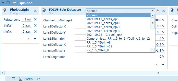
Expand out the PhoibosSpin window, then select the Logical Variables tab. Ensure that ShiftX, ShiftY and RotatorLens are set to what you want for your measurement.

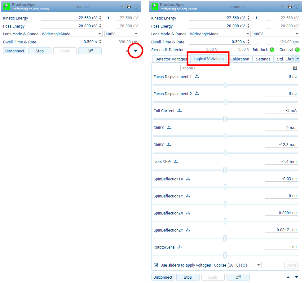
Similarly expand out the FOCUS Spin Detector window, then select the Spin tab:

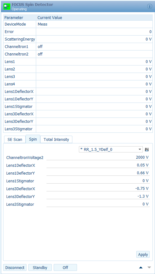
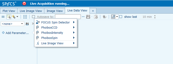
The best intensity monitoring tool for this purpose is the ‘Live Data View’ window:

With Live Data View, choose Add Parameter and then under PhoibosSpin select Count Rate.

Now begin adjusting values. In the PhoibosSpin window, use the bottom dropdown selector to change the adjustment range to Coarse or Medium. Some parameters have very narrow windows, and if you step outside of them the countrate will drop to zero. SD1X (SpinDeflection1X), SD1Y, SD2X and SD2Y are adjusted by dragging the sliders with the mouse. Changes take effect live as you do this. Watch the countrate trace in the Live Data View, and look for the values that give maximum countrate.

In the FOCUS Spin Detector window, L1DX (Lens1DeflectorX), L1DY, L1Stig, L3DX, L3DY and L3Stig are adjusted by clicking on the existing value and typing in a new one. Changes do not take effect until you press ‘Enter’ on the keyboard.

Using the optimized lens voltages

Values for the spin detector (L1DX etc) can be saved to a configuration file by clicking the small disk icon just above where you were editing the values. Those files are stored in C:\ProgramData\SPECS\SpecsLab Prodigy\Devices\FOCUSSpinDetector\Spin and can be viewed in any plain text editor.

Values for the transfer lens (S1DX etc) can likewise be saved from the PhoibosSpin device window, but only if you have disabled the ‘Users sliders’ checkbox at the bottom of the Logical Variables tab. These configuration files are stored in C:\ProgramData\SPECS\SpecsLab Prodigy\Devices\Phoibos1D\Logical Variable Settings.

Whenever you are setting up a spin measurement in the Experiment Editor, you need to be sure about what voltages are being used. Don’t ever assume that it will default to sensible values. There are two ways to do this.

For the FOCUS Spin Detector, you can either manually specify all the voltages right in the setup panel, OR you can populate those fields by loading a configuration file that you saved previously:

For the PhoibosSpin settings, it does not seem possible to load values from a config file within the experimental editor. Instead, add all four as logical variables. By default, these will be set to whatever is currently configured in the PhoibosSpin device window, i.e. whatever they ended up as during your last optimization. But you can also manually specify different values here - for example if you want to program a series of measurements that will each require different lens voltages.