DA30-L electron analyzer

Camera	Basler scA 1400-17gm (ICX285AL sensor, 12bit 1392x1040), 17fps
Work function	4.34 eV (Checked 2023.08.28)
Working distance	34 mm
Mean radius	200 mm
Configuration	High pass mode*

*Changing between high pass and low pass modes involves changing some cables on the SES electronics rack. The analyzer is usually left configured in high pass mode in order to access all pass energies - we have so far never observed any improvement in resolution by going to low pass mode.

Deflection mode

Good:

• Record E-k_X-k_Y datasets without moving the manipulator, which means fixed polarization geometry and no risk of moving the light spot to a different part of the sample

• Take fast constant energy surfaces to check sample alignment, without the added confusion of manipulator backlash

• Vary what is effectively the polar angle while watching live in voltage calibration mode

Bad:

• Only the polar angle can be changed electronically. The other deflection axis (tilt) only shifts the spectrum across the detector, it doesn’t bring in any new information. (The tilt functionality is mainly useful for spin-arpes systems where you need to send a specific feature into a small transfer aperture).

• Angle acquisition range is limited compared to a motor scan.

• If the focus is poor, the spectrum will be distorted, and if using an apertured exit slit also cropped. More about this below.

• As the retarding ratio (E_K/E_P) increases, there will be increased cropping. This can force you to use a higher pass energy than you might have liked, so you need to compensate with a smaller analyzer slit.

Focusing

For optimal performance of the analyzer, the illuminated part of the sample must be positioned at the analyzer focus in all three directions (perpendicular to the entrance slit, parallel to the entrance slit and towards/away from the analyzer).

The DA30L is relatively relaxed about working distance (i.e. towards/away from the analyzer) - anything within 0.5mm of optimal is OK. The beamline has been configured to put the light spot close to the analyzer focus, so in practise you have little control over this. If you are getting a sensible signal, the working distance is OK.

Focus parallel to the slit is traditionally accomplished by ‘centering the stripe’ on the detector in transmission mode. Given the geometry and optics at BLOCH, you have no control over this. It should always be centered; changing it would require raising or lowering either the analyzer or the 1.5GeV ring.

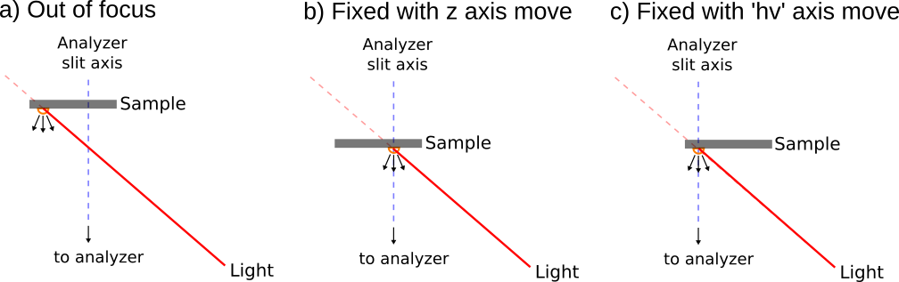
Focus perpendicular to the slit is what you need to work on at Bloch. Typically this is accomplished by fine tuning the manipulator ‘z’ position, although this will move the light spot on the sample. For cases where this is a problem, a virtual ‘hv’ axis is available which will move the sample along the path of the beam. The following diagram schematically depicts the situation as viewed from above:

To first order, the best method of getting into focus is to watch the spectrum in transmission mode and move coarsely (0.1 mm steps) until a well defined stripe begins to appear. Once it does, maximise the count rate with fine steps (e.g. 0.01 mm).

Typically this is good enough. However it is important to be aware that the analyzer focal position is expected to vary slightly with lens mode, pass energy and the presence of any electric fields around the sample. A superior focusing method, albeit a lot more work, is to configure the angular lens mode and pass energy you intend to measure with, then use the deflectors with an apertured analyzer slit to optimize focus. If the alignment perpendicular to the analyzer slit is imperfect, the cropping of the spectrum at high deflection angles will be asymmetric (e.g. you might getting intensity on the detector over +/-6 degrees at +10 degrees deflection, but only +/-2 degrees at -10 degrees deflection). This only works with apertured analyzer slits.

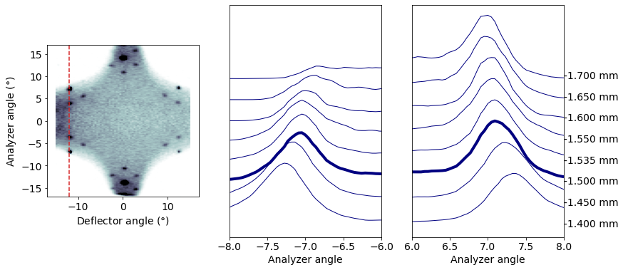
Here is an example using graphene. In this case optimal focus is around z=-1.5mm, based on the symmetrical intensity distribution. You can see how the distribution becomes asymmetric for large deflection angles as you move away from optimal focus.

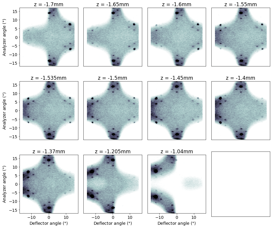
In this particular case, using the easy method of just optimising the transmission stripe would have resulting in using z = -1.4mm. This is not perfect but in most cases would be considered acceptably close.

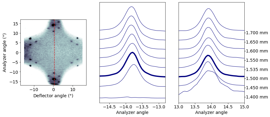
Besides cropping of the spectrum, energy shifts and angular distortions are also expected to be present, particularly at large angles and particularly when the focus is not optimal. Below we extract profiles from the energy surfaces to determine the separation of the Dirac cones. At zero deflection there is almost no distortion no matter how bad your focusing is:

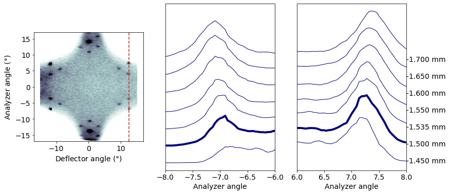
But at high deflection angles this is no longer the case; the angular separation of the Dirac points shrinks or expands as we move away from optimal focus:

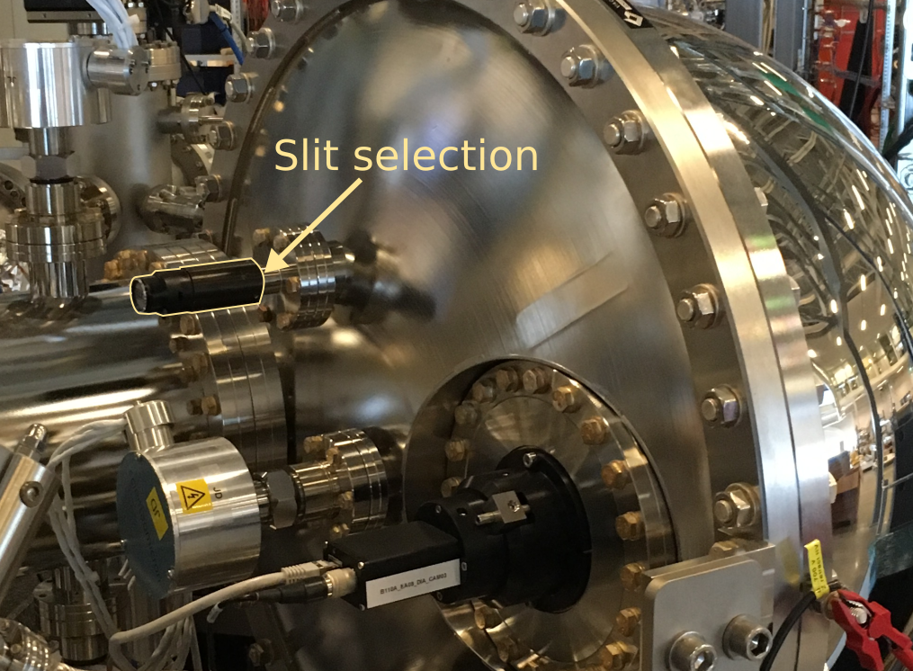
Analyzer slit selection

Change the analyzer slit with the encoder knob on the analyzer. It ‘clunks’ into position when you have reached a slit position. The current value is displayed on the face of the knob.

Encoder index	Slit
100	0.1 mm
200	0.2 mm
300	0.3 mm
400	0.2 mm, with aperture (has artifacts!)
500	0.3 mm, with aperture
600	0.5 mm, with aperture
600	0.8 mm, with aperture
800	1.5 mm, with aperture
900	0.5 mm

All slits are straight. The resulting curvature in the spectrum is automatically corrected by SES. Curved slits sample a curved line in angle-space, and are hence suitable for XPS but not ideal for dispersive bandstructure measurements

Some slits have an aperture installed. The aperture serves to physically mask off electrons that might be entering the hemisphere from the lens at unusual angles. These stray electrons can create problems in all lens modes, but are in practice are only a serious nuisance in transmission modes.

• In transmission mode, energy resolution is noticably better with an aperture (e.g. 5meV for aperture vs 12 meV without, using 0.2mm / Ep5)

• In DA angular lens modes, the aperture has no observable impact on resolution, but it will physically mask ‘bad’ (energy shifted) regions from a deflector map

Lens modes and restrictions

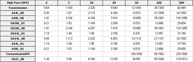
Lens table restrictions

The table below lists hard limits to the lens tables, but also note that the analyzer performs best with a retarding ratio (E_K/E_P) close to 1. Too high and you can’t focus them in time, so there tends to be more of a cutoff effect from stray electrons not making into the hemisphere (particularly for small (<0.3mm) analyzer slits. Too low and the focus is astigmatic, which can lead to angular warping.

The valid kinetic energy ranges for each lens mode are described here: (table also available in SES)

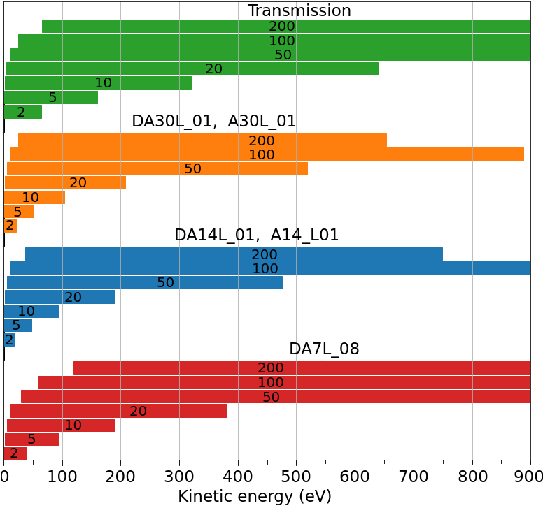
‘_01’ vs ‘_08’

‘_01’ lens modes are configured for small (e.g. synchrotron) spot sizes, while ‘_08’ modes are optimized for large spots (e.g. He lamp). Stay with the ‘_01’ lens mode unless you need DA07, for which we only have _08.

Transmission vs. angular lens modes for core level spectroscopy

Since the transmission lens mode optimizes total photoelectron throughput, it is common in XPS to use transmission mode for measuring core levels. A spectrum measured in transmission mode will have nearly four times the countrate when compared to the same measurement taken in A30L mode. However this is disregarding the importance of keeping the MCP undamaged in an ARPES instrument. Angular lens modes are much better in this respect since they distribute the intensity across the entire MCP instead of dumping it all in an intense central stripe. Unless you have no choice, use an A30 mode to measure core levels. Often with core levels you are limited by the safe count-rate on the detector, so the lost factor of 4 in efficiency when using an angular mode can often be more than compensated by the higher allowed total countrate in angular modes (10e6 vs 1e6)

Fixed vs. scanned/swept acquisition mode

Fixed mode leaves the energy scale fixed and just integrates the image on the CCD. This the most efficient way to collect a Fermi surface map, however the DA30-L has a field-termination mesh in front of the MCP which will show up as a background in your image. In constant energy surfaces this can be quite effectively removed by energy-averaging over a few pixels. But nice looking E-k cuts and in particular quantitative lineshape or disperson analysis is almost impossible in fixed mode.

Swept mode avoids this by translating every part of the spectrum over every part of the detector, which averages out the mesh in the final image.

Another consideration is the kinetic energy range you can acquire: fixed mode is stuck at 7.9% of the pass energy. So:

Pass energy	Energy window in fixed mode (eV)
2	0.16
5	0.40
10	0.79
20	1.58
50	3.96
100	7.91
200	15.82

Deep scans with high energy resolution therefore usually require swept mode.

Mesh suppression

It is possible to greatly suppress the appearance of the mesh in fixed-mode measurements by adjusting the retardation voltage (applied between the grounded mesh and the front of the MCP stack). With zero retardation voltage, incoming electrons striking the mesh are blocked from the MCP and the mesh appears quite strongly in the resulting images. With the default setting of -0.7*Ep, the electrons are slightly defocussed after passing through the mesh which helps to smooth out the resulting image.

A non-standard retardation value of -0.3*Ep greatly reduces the appearance of the mesh, as shown in the example measurements below. These were acquired with hv=180eV, Ep=20eV and normalized to integration time.

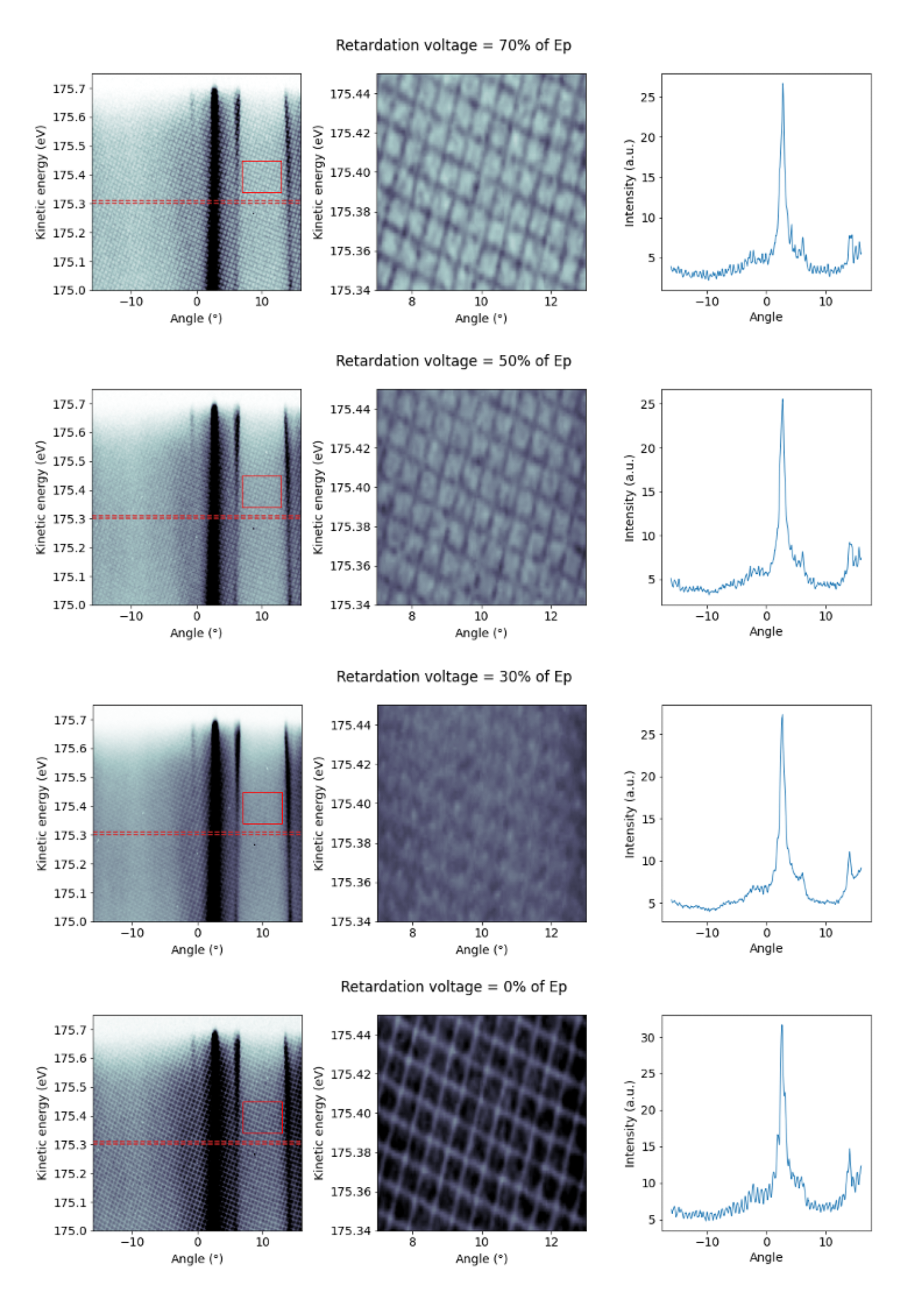
The retardation voltage needs to be set for each pass energy separately. We recommend using being conservative and using the default retardation voltages for swept-mode measurements, since the effects on background and resolution have not been exhaustively characterized.

Angular resolution

The DA30 is nominally capable of <0.1deg angular resolution. In practice it is very rare to find samples with features narrow enough to test this. For now we can say:

Lens mode	Angular resolution (deg)
DA07L_08	< 0.2
DA14L_01	< 0.2
DA30L_01	0.2

Note that wider lens modes have higher photoelectron throughput even after cropping to the same angular range. For example, a given feature measured in A30L is more intense than the same feature measured in A14L by a factor of 2-3, and more intense than when using DA07L by a factor of 4-6.

Energy resolution

Instrumental energy broadening in your measurement has contributions from several different sources (analyzer settings, beamline settings, noise & grounding, magnetic fields …).

A useful property of Gaussian functions is that the convolution of n Gaussians gives another Gaussian with width equal to the quadrature sum of the the input Gaussian widths. On this basis, the final instrumental energy resolution that applies to measured data is:

\[\Delta E = \sqrt{\Delta E_{Analyzer}^2 + \Delta E_{Beamline}^2 + \Delta E_{Noise}^2}\]

This is only the instrumental resolution. Your sample can contribute additional broadening depending on the physics involved (disorder, phonon interactions etc). Cooling down will often sharpen up the bands in your sample, but it has no effect on the instrumental resolution

The beamline or analyzer can usually always be adjusted for higher energy resolution, but it costs intensity. In general the optimal situation is to balance the beamline and analyzer contributions. For example, if the analyzer resolution were >50meV then it would be counterproductive to squeeze the beamline resolution down from 10meV to 5meV - you would be throwing away intensity for almost negligible gain. A resolution calculator is available within pesto to help you plan your measurements.