Phoibos 150 electron analyzer

Camera	PCO pixelfly PF-Q-ME (ICX285AL sensor, 14bit 1392x1040)
Work function	4.5694 eV (FAT)
Working distance	35mm
Mean radius	150 mm

Deflection mode

Only possible in fixed mode. ShiftX simulates a polar rotation (perpendicular to analyzer slit), ShiftY simulates tilt (along analyzer slit).

Spin detector

Overview

At the exit of the hemispherical analyzer the electrons can either be directed to the MCP/CCD stack like a usual ARPES instrument, or they can be directed through an aperture into the spin-detector system. This consists of various electrostatic lens elements and a magnetic rotator that acts on the transverse component of the spin polarization vector, followed by an electrostatic 90 ° deflector into the Ferrum VLEED detector.

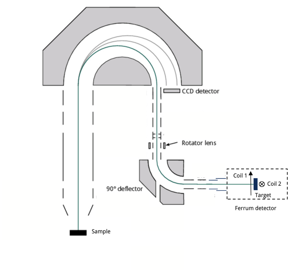
The VLEED (Very Low Energy Electron Diffraction) detector is based on the asymmetric exchange scattering of low energy electrons from a magnetized target, in this case an oxidized 60ML (10nm) Fe film grown on a W(001) crystal. This target has easy magnetization axes along the in-plane [001] directions, and can be initialized with helmholtz coil pairs. This offers spin-sensitivity along two polarization axes. The third polarization axis is accessed with the help of the spin rotator, as will be explained below.

The scattering target is fixed within the detector, and is flashed and re-prepared in-place.

The VLEED detector has two different channeltrons that can be measured. Total intensity is measured by deflecting the beam into the first channeltron, without scattering from the target. The second channeltron records the scattered signal. It is not possible to measure both signals simultaneously, nor is it possible to record spectra on the CCD simultaneously with spin-ARPES spectra.

Measurement principle

The images below indicate the measurement geometry. We see the trajectory of photoelectrons leaving the sample (right), passing through the analyzer and impacting the target (left). In all cases the target magnetization, indicated by an orange arrow on the target, is shown in the ‘positive’ direction.

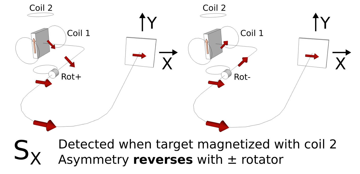
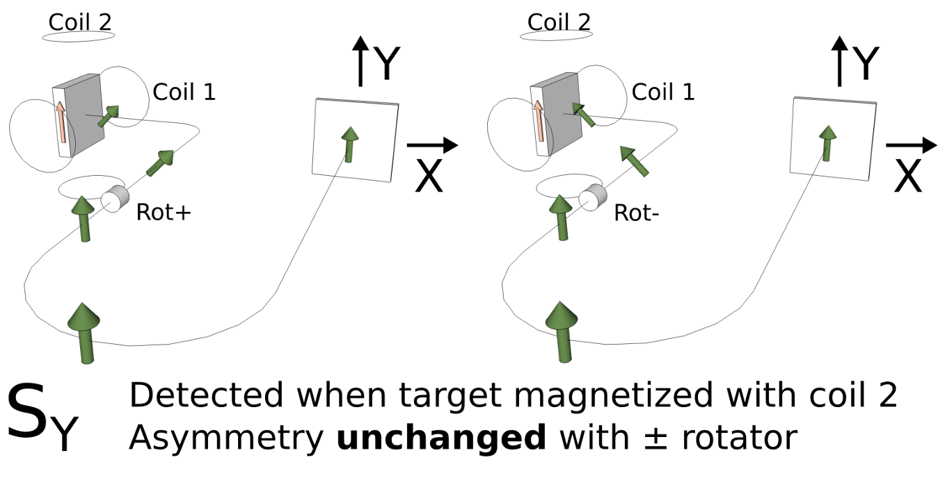
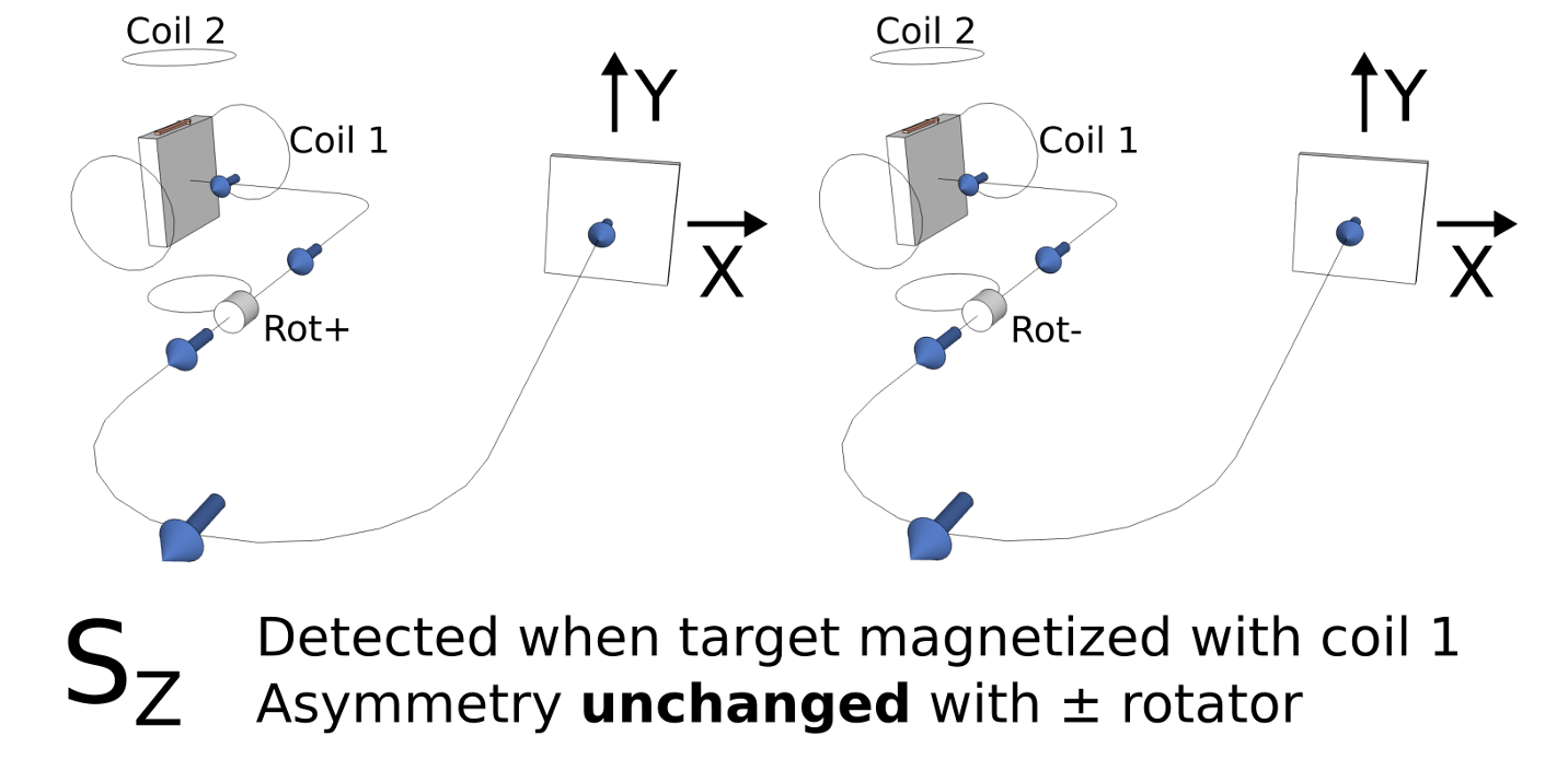
The spin rotator should always be engaged, even if the measurement does not call for it (e.g. coil 1) since the rotator also has a focusing effect.

Angular and energy resolution

The spin detector has selectable circular apertures (diameter 7mm, 3mm, 1mm, 0.5mm) that, together with the hemisphere settings, define the angular and energy resolution of a spin measurement. Below we see the spin aperture below the MCP, for the four different aperture settings.

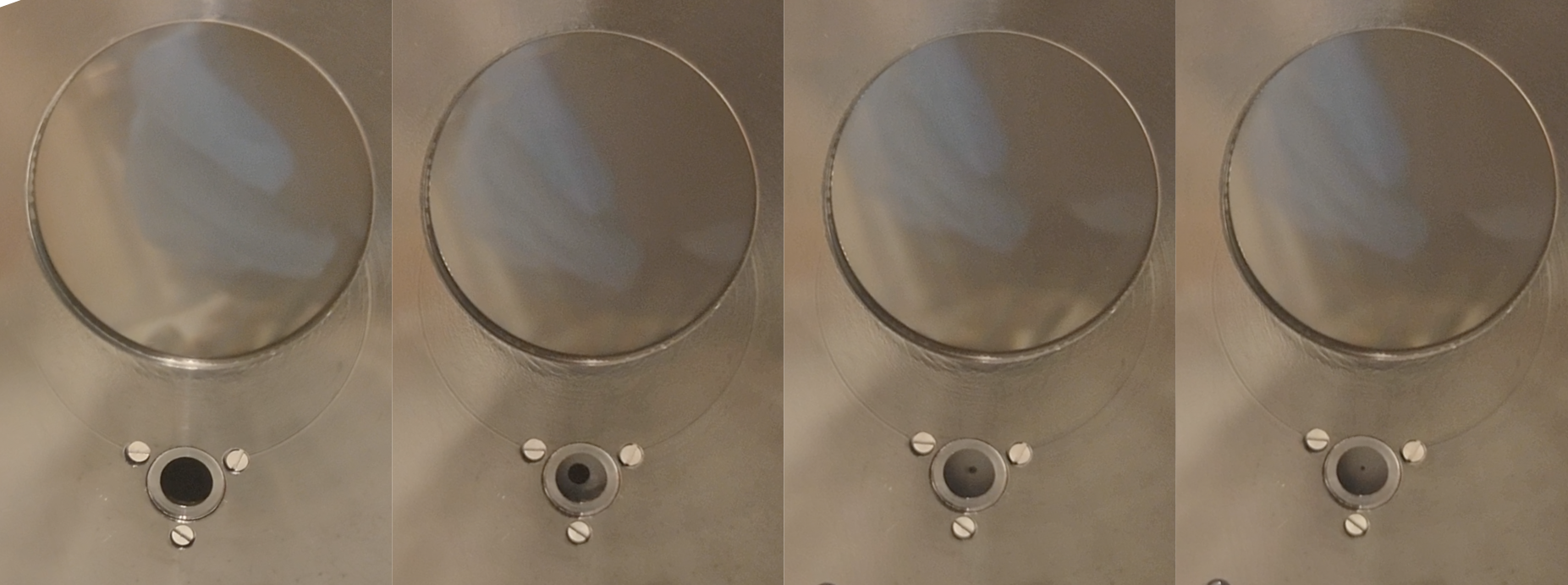
Angular resolution: The analyzer entrance slits are 20mm wide. This means an x mm aperture will accept the middle x/20 of whatever image the CCD is currently seeing

Mode	7mm	3mm	1mm	0.5mm
HAD (± 3 °)	2.1	0.9	0.3	0.15
MAD (± 4 °)	2.8	1.2	0.4	0.2
LAD (± 7 °)	4.9	2.1	0.7	0.35
MAM (± 10 °)	7	3	1	0.5
WAM (± 15 °)	10.5	4.5	1.5	0.75

Energy resolution: This follows a similar argument, except now we consider that the aperture is accepting x/35 of whatever energy range the MCP is currently accepting (which is given by Ep * 0.10). 35mm corresponds to the active area of the MCP.

That gives us, in meV:

Epass	7mm	3mm	1mm	0.5mm
5	100	43	15	7
10	200	86	39	14
20	400	171	57	29
30	600	257	86	43
40	800	343	114	57
50	1000	430	140	71

This calculation does not account for other sources of broadening. If the best resolution you can obtain with the CCD is 30meV, you will never do better than 30meV with any spin detector settings. Also: the aperture is a circle, not a square, so the energy and angle resolutions should be slightly better than these estimates. Finally, remember that energy and angle resolution convolve if you are measuring dispersive bands (i.e. bad angular resolution on a steep band results in bad energy resolution)

Experimentally measured energy resolution values from an Au foil fermi edge at 78K (Sept 2023) are:

Epass	7mm	3mm	1mm	0.5mm
5
10		58	32	30
20		127	56	48
30		223	87
40		284	106
50			132	110

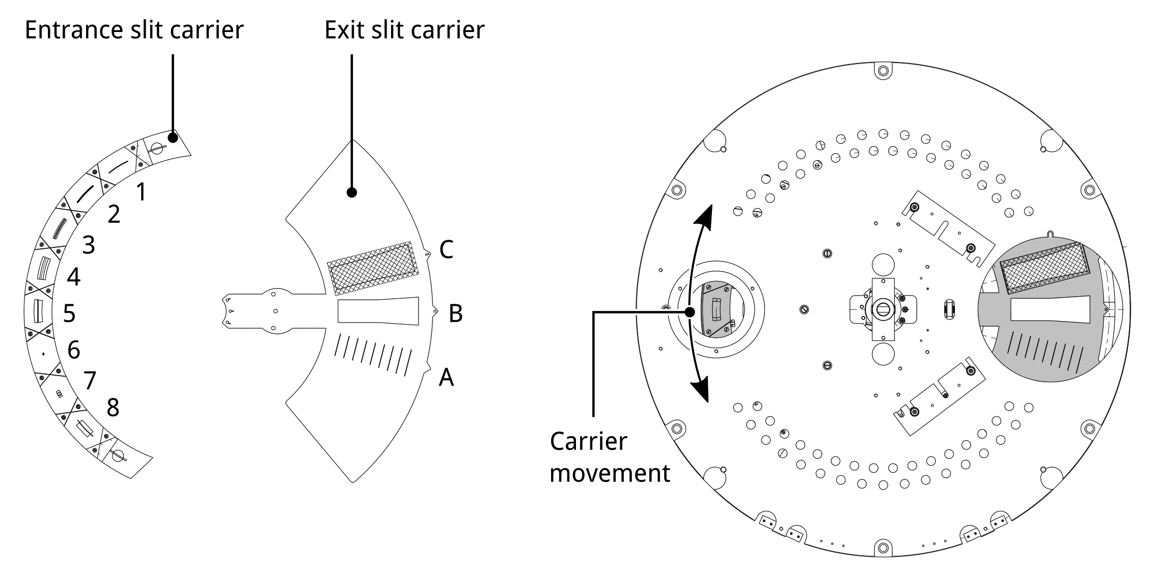
Analyzer slit selection

Slit number	Slit width (mm)
1	0.05
2	0.05
3	0.1
4	0.1
5	0.2
6	0.5
7	0.8
8	3mm diameter aperture

All slits are straight, with the resulting curvature automatically corrected by Prodigy. Change the exit slit with the encoder knob on the flat face of the analyzer (if you dare). The indicators on the knob are unreliable, but if in doubt you can verify by watching how the intensity changes as you move through positions.

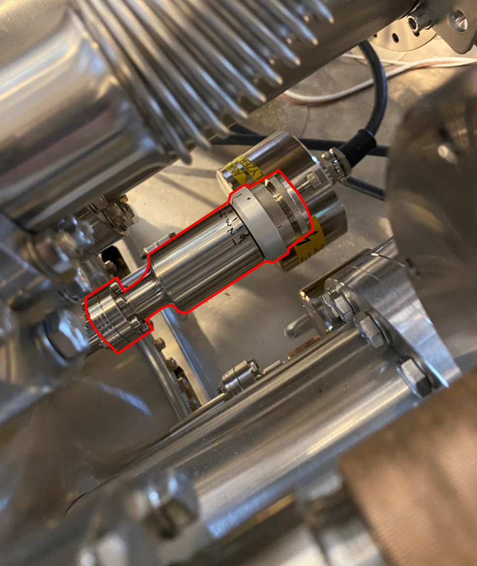
One important quirk to be aware of with the mechanism is that continuing to rotate past the end points will actuate a second, slit carousel in front of the MCP. In most cases this will not be what you want, and you will have to rotate all the way back to the other extreme of the slit carousel to push it back.

Spin aperture selection is subtle and difficult, and is only recommended to be performed by beamline staff.

Energy resolution

Instrumental energy broadening in your measurement has contributions from several different sources (analyzer settings, beamline settings, noise & grounding, magnetic fields …).

A useful property of Gaussian functions is that the convolution of n Gaussians gives another Gaussian with width equal to the quadrature sum of the the input Gaussian widths. On this basis, the final instrumental energy resolution that applies to measured data is:

\[\Delta E = \sqrt{\Delta E_{Analyzer}^2 + \Delta E_{Beamline}^2 + \Delta E_{Noise}^2}\]

This is only the instrumental resolution. Your sample can contribute additional broadening depending on the physics involved (disorder, phonon interactions etc). Cooling down will often sharpen up the bands in your sample, but it has no effect on the instrumental resolution

The beamline or analyzer can usually always be adjusted for higher energy resolution, but it costs intensity. In general the optimal situation is to balance the beamline and analyzer contributions. For example, if the analyzer resolution were >50meV then it would be counterproductive to squeeze the beamline resolution down from 10meV to 5meV - you would be throwing away intensity for almost negligible gain.