Using SES to measure

Measurements at Bloch are taken through Scienta’s ‘SES’ software, v1.9.2. You will find a shortcut to it on the desktop.

Preliminary notes about SES:

Regions, sequences and iterations

All measurements happen by configuring them in the sequence editor, then running the sequence.

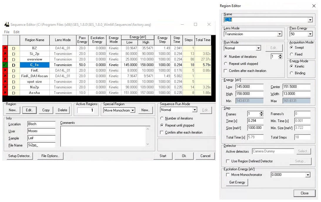
When programming a measurement in the sequence editor, SES offers several layers of hierarchy. The terminology can be confusing:

A sequence is a list of measurements you wish to perform. Each entry in that list is called a region. Some types of regions can have more than one iteration (or what we might call sweeps).

Programming a complicated multi-measurement sequence is common for XPS, but in ARPES it is more common to have only one active region in the sequence at a time. Typically one might like to leave that measurement integrating indefinitely, manually stopping when you are satisfied with the quality. There are different permutations that accomplish this, but they are not all equivalent!

The most important difference is that the measurement is saved to disk when a region is completed. This means that if you set multiple region iterations, nothing will save until it has finished (either naturally or by you asking it to stop).

Advantage: Less time spent writing to disk

In contrast, if you set the iterations at the sequence level, the measurement will be saved after every iteration.

Advantage: Data is safer against SES crashes

Advantage: You can access the data in external analysis software while SES continues to update it in the background.

If you really want to break your long DA30 scan into multiple iterations, there is a way around this. If the sequence contains multiple identical DA30 scan regions, you will end up with one zip file containing several .bin files. You would then be able to manually combine them if desired. It is not saved until the end, so you can’t look at it while it measures.

File formats

When configuring the savefile path (File Options in sequence editor) you can also choose which file formats to save to. DA30 scans are always and only .zip files, but everything else can be any or all of (.pxt, .ibw and .txt). Choose whatever your analysis software takes, but note that large scans (big manipulator maps or hv scans) saved to txt can cause memory issues and crash SES. Don’t save to txt unless you really need it. You can always use SES to convert between file formats afterwards.

Deflector ARPES scans

See also the discussion on the see DA30-L electron analyzer page), especially regarding focusing, exit slit aperture and fixed vs. scanned modes.

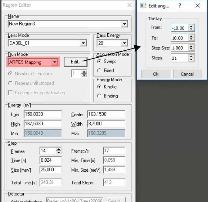
Comments:

SES does not automatically rezero the deflectors when it completes a DA30 angular map! Manually re-zero it using the DA30 menu in the main SES window.
Fast DA30 angle maps (2-3s/frame in fixed mode) combined with the pesto ‘align’ function are a useful method of quickly evaluating and correcting the angular alignment of your sample.
View measurements in pesto with pesto.explorer(“filename.zip”)

1D manipulator scans (e.g. Fermi surface maps)

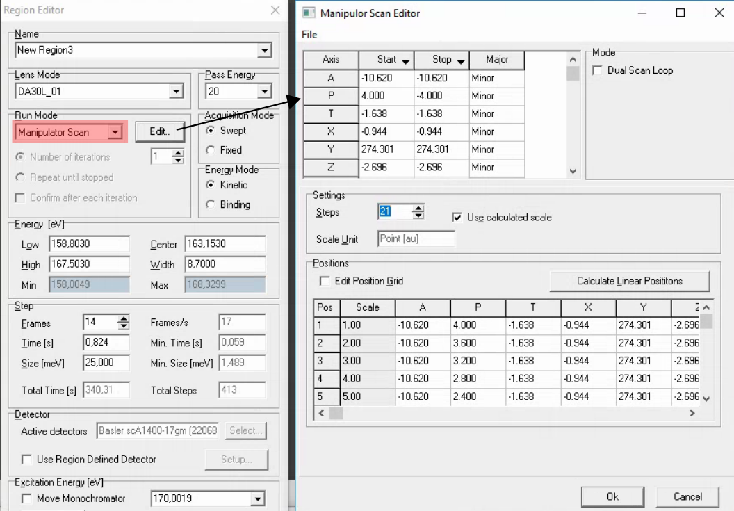
Comments:

You can right click on the ‘Start’ and ‘End’ cells in the top row to set to the current manipulator position. But still always double check that the values are correct, and always check that any axis that shouldn’t be moving has the same starte and stop value.
Don’t forget to mark the axis you are scanning as a major axis
If it is a polar scan and the range is more than 5-10 degrees, in order to maintain reasonable focus you will need to be close to the manipulator center of rotation (approximately x=0.185) and you may need to scan z along with polar.
Nothing is saved until the end, and the SES viewer unhelpful just concatenates all scans. It is typically worth first running a very fast version of the measurement to ensure that all settings are correct, that your settings are safe for the highest intensity regions of the scan and that you will get what you want.
View measurements in pesto with pesto.explorer(“filename.ibw”)

Time dependent scans

A hack workaround for time dependent scans is to program a 1D manipulator scan in which the start and end polar values are within 0.01 degrees of each other. The logic layer between SES and the control system filters out any motion requests that are below a certain threshold, so a scan like this will result in no motion at all.

This can also serve as a hack workaround for temperature dependence, if you pair it with a suitably slow temperature ramp. In this case, make sure to save a copy of the temperature log file that is saved to the ControlGUIs folder.

Photon energy scans

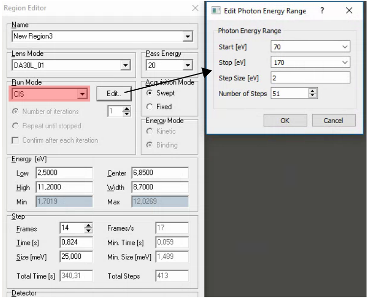
Comments:

This is enabled by a special addition to give SES access to the same ‘beamline energy’ input you control, which simultaneously sets the monochromator energy and EPU gap. It will work for all polarization modes, but you still need to manually toggle between polarizations - changing polarization within SES is not currently possible. (Note for staff: details of the implementation are described in elogy.)
If you just want to measure a few different photon energies, it is also possible to insert a special region in the sequence editor that changes the photon energy
When changing photon energy, SES will wait a certain amount of time (120s) then just move on with the sequence regardless of whether the monochromator has finished moving. At lower energies the monochromator becomes progressive slower to move, so it is generally a good idea to already be at the starting photon energy for an hv scan. For the same reason, when using the special ‘set hv’ region in the sequence editor it can pay to set it twice in a row if there is any risk that 120s will not be long enough to complete the move.
For photon energy scans you will have to specify the measurement range in binding energy. The work function is currently set to zero in SES, so Eb = hv - Ek. The easiest approach is to switch to binding energy scale in voltage calibration mode and read off the start and end values you want to scan over.
Nothing is saved until the end, and the SES viewer unhelpful just concatenates all scans. There is a separate viewer window which shows the angle-integrated spectrum as a function of hv, which can be helpful just to know that something is happening:
It is typically worth first running a fast, coarse version of the measurement to ensure that all settings are correct, that your settings are safe for the highest intensity regions of the scan and that you will get what you want.
View measurements in pesto with pesto.explorer(“filename.ibw”)

2D manipulator maps (e.g. X-Y spatial maps)

Note

It is highly recommended to configure X-Y map regions via the ‘Automap’ control panel instead of configuring them manually within SES.

To scan two manipulator axes, most typically X and Y for a spatial map, check the ‘dual scan loop’ box when setting up a manipulator scan. You can now choose two major axes and assign one to the inner and one to the outer scan loop.

Comments:

It is a good idea to talk to one of the beamline staff before first attempting one of these measurements - there are several special considerations to keep in mind
The ibw data format used by SES is fundamentally incompatible with file sizes larger than 2Gb. If your scan exceeds this, it will be corrupted. As a general rule of thumb, 20x20 maps will work when acquiring full-frame fixed mode images. To make larger scans, you will need to enable angle binning and/or reduce the detector frame size in order to produce smaller files. You can configure this from the main window in SES under Setup>Global detector. Binning is enabled by setting the ‘Slices’ field to some integer fraction of the maximum, e.g. 400 slices out of a possible 800 corresponds to binning by a factor of two. XPS maps in transmission mode can use aggressive binning without any compromise. Remember to return to full resolution settings after the map!
It is highly recommend to set up 2D scans from the ‘Automap’ panel instead of configuring them manually within SES. When loading the sequences files produced by that panel, a bug in SES will usually corrupt the final position list. You must force SES to recalculate it by changing the number of points in the inner and outer loop (i.e. increment by one then decrement by one)
There is a preferred scan direction (positive) to avoid triggering backlash compensation every step. In the Automap panel this is accomplished by dragging from upper right to lower left when defining the scan region.
These measurements involve a lot of measurements and so take a long time. Scanned mode ARPES is often infeasible, so use fixed mode wherever possible.
Step sizes down to approximately 10μm in X and Y are reasonable. Steps below 5μm start to exceed the capabilities of the XYZ stage and can be unreliable.
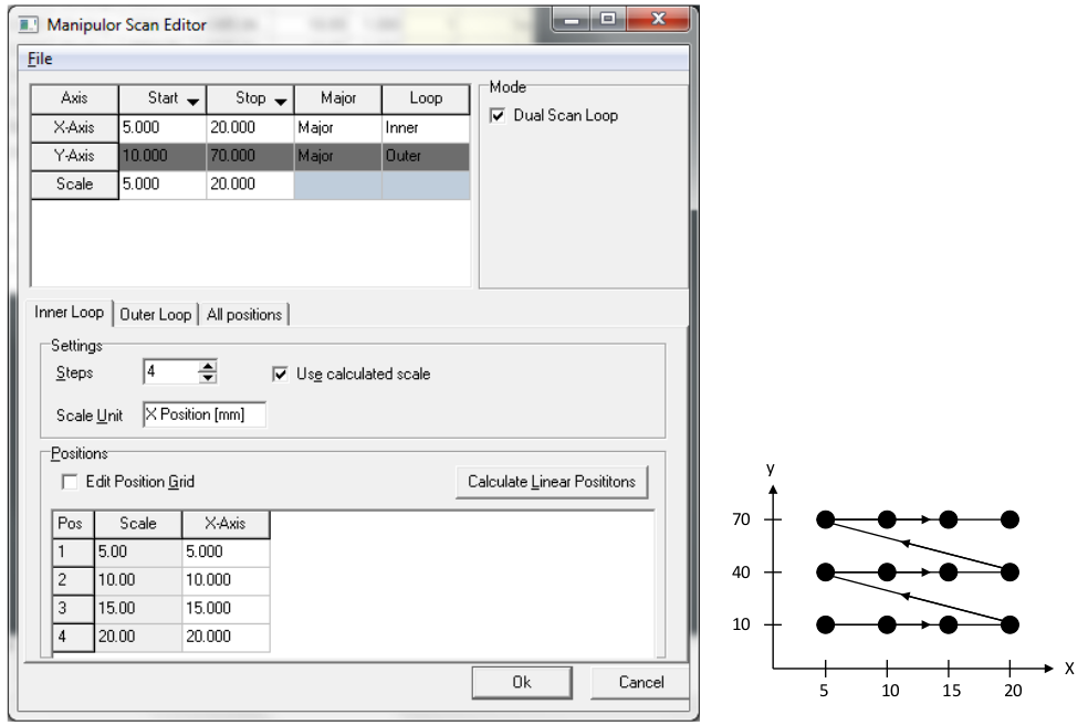
If configuring the scan manually in SES: You can right click on the ‘Start’ and ‘End’ cells in the top row to set to the current manipulator position. But still always double check that the values are correct, and always check that any axis that shouldn’t be moving has the same starte and stop value. Check this on each of the ‘inner loop’, ‘outer loop’ and ‘all positions’ tab - SES will try very hard to trip you up, so be vigilent.
Data can be viewed in pesto with pesto.explorer(“filename.ibw”)