How to measure

Maximum countrate

Excessive countrates will damage the MCP in the detector assembly, and at BLOCH it is very easy to generate unsafe countrates. Respect the following rules:

1. Maximum 1 million counts/s if everything is in a narrow stripe (for example transmission mode or graphene’s Dirac cone)

2. Maximum 10 million counts/s if intensity is evenly distributed across the detector

3. Core levels should be measured in an angular lens mode, except where lens table limits make this impossible.

Warning

There is no background process in SES to monitor countrates, so you must verify that the countrate is safe while in voltage calibration mode. If you will perform an angle scan or photon energy scan, check the intensity over the whole scan range, not just your starting position. If you will measure in swept mode, ensure that the intensity slightly below your starting point is also safe.

Control GUIs

How to launch control GUIs

For the control panels on the ‘Scienta’ spectrometer control computer (Windows), there is a folder on the desktop of the measurement computer called ‘ControlGUIs’. Within this you will find all of the control GUIs discussed below. All of them have a corresponding ‘Launch’ shortcut you can double click on.

For the control panels on the ‘beamline’ control computer (Linux) there is a ‘Bloch controls GUI’ shortcut on the desktop that brings up a launcher for all the sub-panels.

There is some redundancy between what you can do with the controls on the two different computers. As a general rule, the panels on the Linux computer are more full featured while those on the Windows computer are simplified to the bare minimum required to perform an experiment. Those who are measuring remotely through a VPN connection can only access the Windows computer.

Beamline control panel (Windows computer)

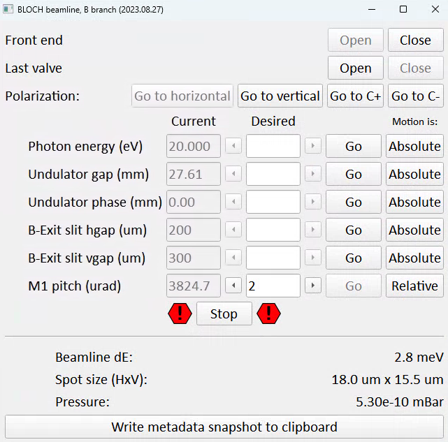
Front end and last valves

‘Front end’ here refers to the set of valves and shutters immediately following the undulator. They will automatically close if there is an interlock condition or a beam dump.

‘Last valve’ is the final pneumatic valve isolating the endstation from the beamline. Remember to close it as a precaution if you are transferring or annealing samples.

Whenever you are not using the beam for an extended period, leave the last valve and front end closed as precaution.

Setting polarization

Horizontal polarization means an undulator phase of 0mm, while vertical polarization is a phase of 42mm. The polarization buttons on the control panel will change the undulator phase, then ‘wobble’ the photon energy up and down by 0.1eV to force the beamline to set the correct undulator gap.

Circular polarization is currently set manually, with the aid of a separate calculator GUI that is also launched from the same folder.

Setting photon energy / polarization

Requesting a photon energy will automatically configure the monochromator, undulator and M1 pitch correctly (more on M1 pitch below). For all of these entry fields you need to click ‘Go’ before anything will happen, pressing the enter key will not do anything.

The undulator gap and phase are exposed on this panel, but when using linear polarization modes there is usually no need to interact with these.

Exit slits

The exit slit horizontal gap determines energy resolution, vertical spot size and flux.

The vertical gap determines horizontal spot size and flux.

The settings here are typically dictated by getting the resolution you want while limiting the flux so that the detector is not damaged. When measuring ARPES typical values are (100μm x 100μm), but it is not unusal to need to close down to (20μm x 100μm) or lower purely to avoid damaging the detector. Aligning the sample in transmission mode requires settings more like (15μm x 15μm). If you don’t care about spot size, flux will continue to increase for vertical gap values up to around 700μm, and the same for horizontal gap if you don’t care about energy resolution.

The estimated beamline resolution and spot size on the sample is estimated at the bottom of the panel based on your current settings.

M1 pitch

One of several functions of the first mirror (‘M1’) is to deflect the beam horizontally. If the mirror pitch is not optimized, the beam does not ‘thread the needle’ through the downstream optics and photons are needlessly lost. M1 pitch is set automatically based on an empirical lookup table, but since the issue is heatload dependent this is not usually perfect. You will often see substantial flux gains by optimizing it. Whenever you change photon energy, adjust M1 pitch while watching the countrate - the lineshape is gaussian and the optimal position should be obvious.

At low photon energies (< 18eV) where there is a high heat load from the undulator, the optimal M1 pitch can unfortunately become time dependent.

If the default lookup values are badly off and this is ruining things like automatic photon energy scans, it is possible to quickly (5mins) recalibrate the lookup table. This is a work in progress, so discuss with beamline staff to get the latest advice.

Write metadata snapshot to clipboard

This is a convenience function to work around the dearth of beamline metadata saved by SES. Besides analyzer and scan settings, currently only manipulator position and photon energy are saved in measurement metadata. Pressing this button will paste a metadata string to the clipboard, which you can then paste into the comments field in the sequence editor. SES does not allow ‘ctrl+v’ pasting, you need to right click and select paste.

Manipulator control (Windows computer)

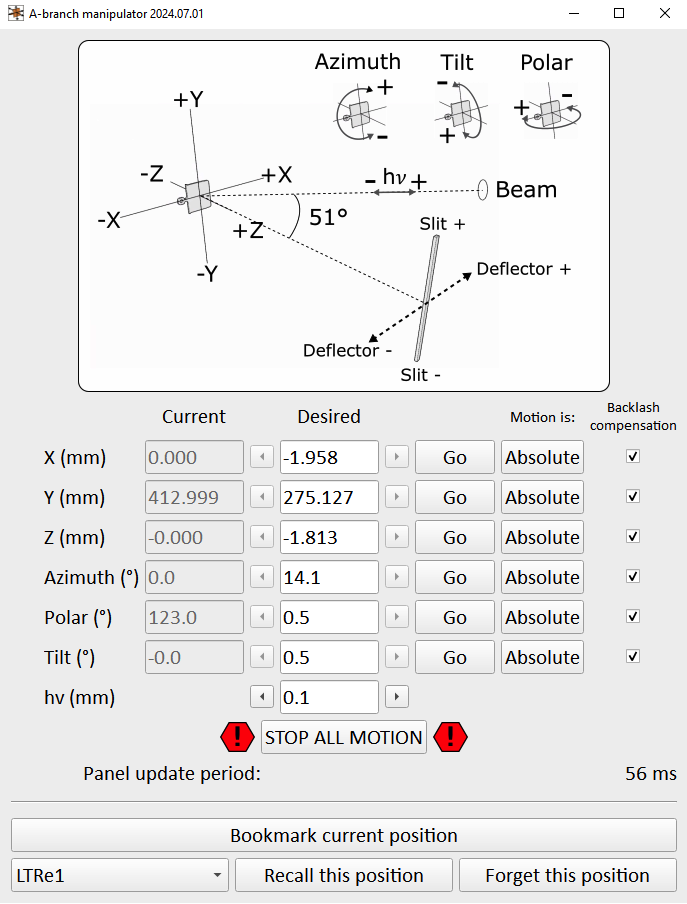
This panel controls the Carving 6-axis manipulator motion. Axes can be toggled between relative and absolute motion, and nothing will happen until you click the ‘Go’ button.

The motion in this interface is software restricted to a safe bounding volume, so in principle it should not be possible to crash the manipulator into anything.

You will be using either the z-axis or ‘hv’ axis to bring the sample into focus perpendicular to the slit; start with steps of 0.1 but once you’re approaching the optimal fine tune in steps of 0.02. Focusing is discussed in more detail on the ‘DA30’ page)

If you are scouting around the sample and want to ‘bookmark’ good positions you find, the ‘Save current position’ button will do this. All positions are saved only to memory, and will be erased if the control panel is closed. Pressing the ‘recall’ button for a saved position will populate the ‘Desired’ fields for the 6 axes, but nothing will move until you press ‘Go’ for each of these axes one by one.

You should only need to manually adjust the Carving position when you are measuring - going up and down between the measurement and transfer positions is performed as pre-programmed paths in order to avoid collisions. These motions are currently only possible from the Linux control computer, you cannot do them from the Windows computer.

Temperature control panel (Windows computer)

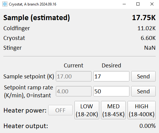
This panel controls the Lakeshore controller which measures the cryostat temperatures and runs the counter-heater. See the detailed discussion on the ‘Carving’ page for information on how to interpret the temperatures shown here. Inputs here are:

Sample setpoint: What temperature you want to have on the sample. Note that nothing will happen if the heater power is set to ‘OFF’

Ramp rate: How fast the sample setpoint is allowed to change

Heater power: Maximum power the control loop is allowed to give the heater. Each button indicates the temperature range that can be achieved for that setting. It is typical to choose either ‘OFF’ (for base temperature) or ‘HIGH’ (anything else)

Trendplots (Windows computer)

Simple temperature and pressure trendplot panels are available. These will only start plotting data from the time they were launched onwards.

Launcher panel (Linux computer)

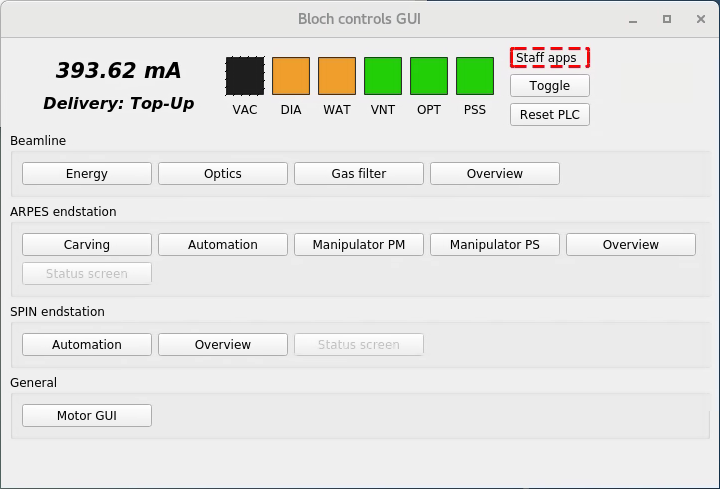
From here you launch other panels with specialized functions. As a user you will be mostly interacting with the ‘Carving’ (manipulator control) and ‘Energy’ (beamline control) panels.

Carving panel (Linux computer)

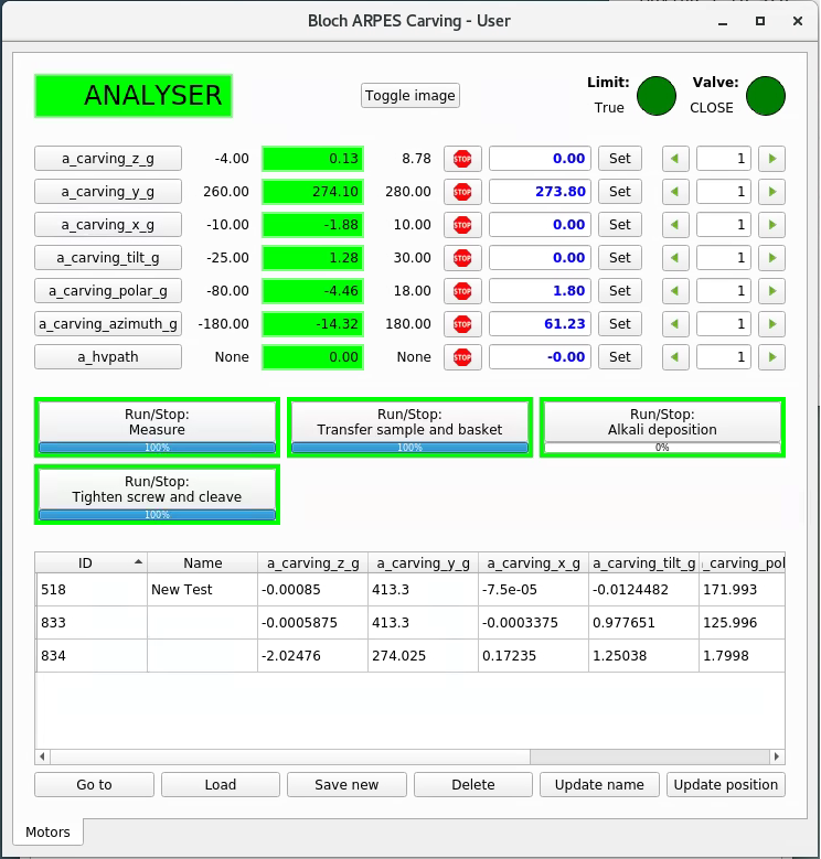
Similar to the ‘Manipulator control’ on the Windows computer, except now you have some additional buttons to initiate movement between the major positions. These are:

Measure	Put the sample in front of the analyzer
Transfer sample and basket	Pick up samples from the transfer arm and insert them into the manipulator
Alkali deposition	Place the sample in front of the alkali source (see Alkali deposition page)
Tighten screw and cleave	Tighten/loosen the two clamping screws on the manipulator, and/or cleave a sample

There are two indicators in the top right of this panel. Both must be green before the movement buttons will work. ‘Valve’ means the gate valve to the transfer chamber (which must be closed). ‘Limit’ means the manipulator position is somewhere abnormal and needs to be manually moved back into a predefined bounding volume. Beamline staff can help you with this.

Warning

Always retract both wobblesticks fully after you have used them. If they are left pushed into the chamber, the manipulator can catch on them and cause major damage when it moves between positions.

Energy panel (Linux computer)

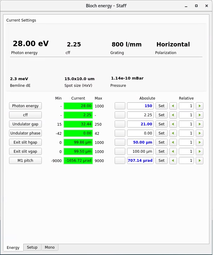
Similar to the ‘Beamline control panel’ on the Windows computer, except now you have some additional options. Among them:

1. You can change the cff setting of the monochromator for higher intensity or higher resolution (proceed with caution, the energy calibration is only checked for cff=2.25)

2. In the ‘Setup’ tab you can change monochromator gratings (discuss with staff first and proceed with caution, only the 800 l/mm grating is fully commissioned)

Optimizing flux

If you need a higher countrate, your options are as follows, in order of preference:

0. Optimize the sample focus and/or find a better place on the sample (free)

1. Fine tune the M1 pitch (free)

2. Use a larger exit slit vgap, up to 800μm (increases spot size)

3. Use a larger analyzer slit or pass energy (lowers resolution)

4. Use a larger exit slit hgap (lowers resolution)

5. Detune the undulator to a slightly higher gap - go in steps of 0.1mm (may worsen higher order contamination)

If you are instead concerned about beam damage and you want a deliberately lower flux, your options are, in order of preference:

0. Close down exit slit hgap, gets weird below 5μm (improves energy resolution)

1. Close down exit slit vgap, gets weird below 5μm (reduces spot size by truncation)

2. Detune the undulator gap

3. Detune M1 pitch

Using SES

Measurements at Bloch are taken through Scienta’s ‘SES’ software, v1.9.2. You will find a shortcut to it on the desktop. Manuals are here (pdf) and here (pdf)

Preliminary notes about SES:

Regions, sequences and iterations

All measurements happen by configuring them in the sequence editor, then running the sequence.

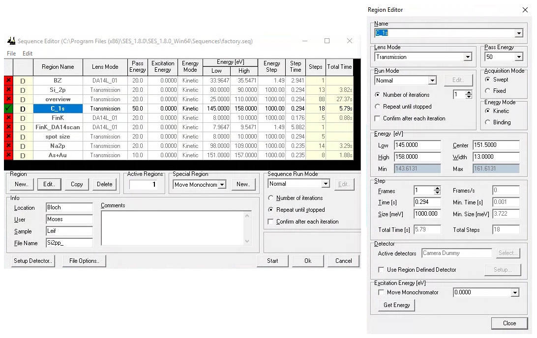
When programming a measurement in the sequence editor, SES offers several layers of hierarchy. The terminology can be confusing:

A sequence is a list of measurements you wish to perform. Each entry in that list is called a region. Some types of regions can have more than one iteration (or what we might call sweeps).

Programming a complicated multi-measurement sequence is common for XPS, but in ARPES it is more common to have only one active region in the sequence at a time. Typically one might like to leave that measurement integrating indefinitely, manually stopping when you are satisfied with the quality. There are different permutations that accomplish this, but they are not all equivalent!

The most important difference is that the measurement is saved to disk when a region is completed. This means that if you set multiple region iterations, nothing will save until it has finished (either naturally or by you asking it to stop).

Advantage: Less time spent writing to disk

In contrast, if you set the iterations at the sequence level, the measurement will be saved after every iteration.

Advantage: Data is safer against SES crashes

Advantage: You can access the data in external analysis software while SES continues to update it in the background.

If you really want to break your long DA30 scan into multiple iterations, there is a way around this. If the sequence contains multiple identical DA30 scan regions, you will end up with one zip file containing several .bin files. You would then be able to manually combine them if desired. It is not saved until the end, so you can’t look at it while it measures.

File formats

When configuring the savefile path (File Options in sequence editor) you can also choose which file formats to save to. DA30 scans are always and only .zip files, but everything else can be any or all of (.pxt, .ibw and .txt). Choose whatever your analysis software takes, but note that large scans (big manipulator maps or hv scans) saved to txt can cause memory issues and crash SES. Don’t save to txt unless you really need it. You can always use SES to convert between file formats afterwards.

Deflector ARPES scans

See also the discussion on the see DA30 page), especially regarding focusing, exit slit aperture and fixed vs. scanned modes.

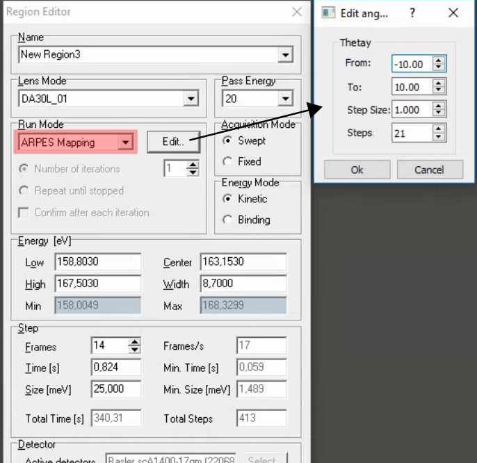
Comments:

• SES does not automatically rezero the deflectors when it completes a DA30 angular map! Manually re-zero it using the DA30 menu in the main SES window.

• Fast DA30 angle maps (2-3s/frame in fixed mode) combined with the pesto ‘align’ function are a useful method of quickly evaluating and correcting the angular alignment of your sample.

• View measurements in pesto with pesto.explorer(“filename.ibw”)

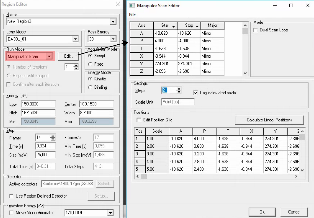
1D manipulator scans (e.g. Fermi surface maps)

Comments:

• You can right click on the ‘Start’ and ‘End’ cells in the top row to set to the current manipulator position. But still always double check that the values are correct, and always check that any axis that shouldn’t be moving has the same starte and stop value.

• Don’t forget to mark the axis you are scanning as a major axis

• If it is a polar scan and the range is more than 5-10 degrees, in order to maintain reasonable focus you will need to be close to the manipulator center of rotation (approximately x=0.185) and you may need to scan z along with polar.

• Nothing is saved until the end, and the SES viewer unhelpful just concatenates all scans. It is typically worth first running a very fast version of the measurement to ensure that all settings are correct, that your settings are safe for the highest intensity regions of the scan and that you will get what you want.

• View measurements in pesto with pesto.explorer(“filename.ibw”)

Photon energy scans

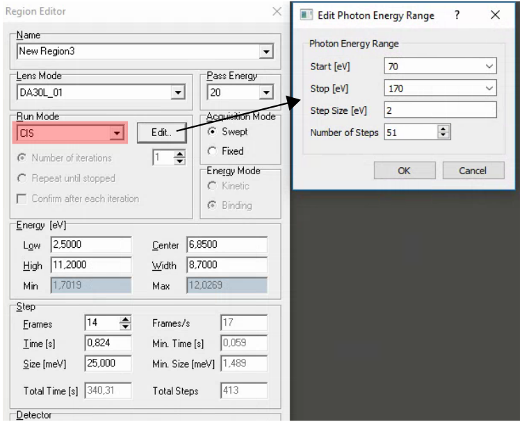
Comments: - This is enabled by a special addition to give SES access to the to the same ‘beamline energy’ input you control, which will simultaneously set the monochromator energy, EPU gap and M1 pitch (using lookup tables). It will work for both vertical and horizontal polarization, but you need to manually toggle between the two modes - changing polarization within SES is not currently possible.

• If you just want to measure a few different photon energies, it is also possible to insert a special region in the sequence editor that changes the photon energy

• When changing photon energy, SES will wait a certain amount of time (120s) then just go for it regardless of whether the monochromator has finished moving. At lower energies the monochromator becomes progressive slower to move, so it is generally a good idea to already be at the starting photon energy for an hv scan. For the same reason, when using the special ‘set hv’ region in the sequence editor it can pay to set it twice in a row if there is any risk that 120s will not be long enough to complete the move.

• For photon energy scans, you will have to work in binding energy (note that the work function is currently set to zero in SES, so Eb = hv - Ek). To check what binding energy range you want to cover, switch to binding energy scale in voltage calibration mode.

• Nothing is saved until the end, and the SES viewer unhelpful just concatenates all scans. There is a separate viewer window which shows the angle-integrated spectrum as a function of hv, which can be helpful just to know that something is happening:

• It is typically worth first running a fast, coarse version of the measurement to ensure that all settings are correct, that your settings are safe for the highest intensity regions of the scan and that you will get what you want.

• View measurements in pesto with pesto.explorer(“filename.ibw”)

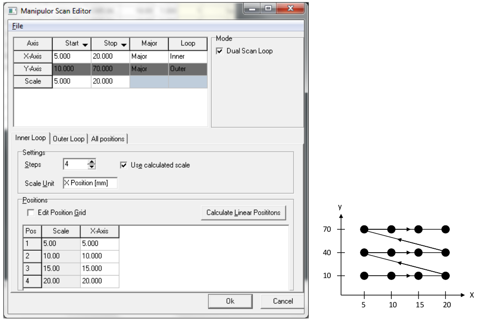
2D manipulator maps (e.g. X-Y spatial maps)

To scan two manipulator axes, most typically X and Y for a spatial map, check the ‘dual scan loop’ box when setting up a manipulator scan. You can now choose two major axes and assign one to the inner and one to the outer scan loop. Since changes in Y couple in an X motion, we recommend scanning with X in the inner loop and Y in the outer loop.

Comments:

• These measurements take a long time, and scanned mode ARPES is often infeasible. However in fixed mode the file size and memory footprint can get quite large. This can cause SES crashes, and also makes the output file difficult to handle in some analysis software. 25 x 25 pixel maps will work. Higher values than this in a fixed-mode map you do at your own risk, although you might consider temporarily reducing the detector frame size (Setup>Global detector) to the minimum that still catches your feature of interest. Remember to set it back afterwards.

• Here are some examples of scan parameters that have been tested and worked without any issues. These do not represent limits, just examples that have worked:

• You can right click on the ‘Start’ and ‘End’ cells in the top row to set to the current manipulator position. But still always double check that the values are correct, and always check that any axis that shouldn’t be moving has the same starte and stop value. Check this on each of the ‘inner loop’, ‘outer loop’ and ‘all positions’ tab - SES will try very hard to trip you up so be vigilent.

• Data can be viewed in pesto with pesto.explorer(“filename.ibw”), but there are other functions available that use alternative methods to generate the image contrast. Discuss with beamline staff if you need some help dealing with these datasets.